Abstract
This chapter introduces the concept of quasi-steady state (QSS) approximations, which provide a means of dimensionality reduction for dynamical systems exhibiting separated timescales. Intuition is developed for timescale filtering effects through examination of a generalized system response equation and specific analytical solutions. A prototypical two-dimensional fast-slow system demonstrates how leveraging clear timescale separation via non-dimensionalization and a QSS approximation reduces the system dimensionality. Comparing the full and reduced systems verifies the approach by showing steady states and stability conditions match under the assumption of large timescale separation. Examining eigenstructure reveals trajectories relax to the slow subsystem, where dynamics are dominated, demonstrating how timescale separation enables analytical tractability. The example establishes the methodology and conceptual foundations for employing QSS approximations to analyze multi-timescale dynamics, which commonly arise across fields including physics, biology and chemistry.
Introduction
Many natural and engineered systems exhibit dynamics that evolve over time governed by underlying mathematical equations. An important class of these dynamical systems involve processes operating on separated timescales, known as multi-timescale systems. In such systems, different state variables respond on distinct fast and slow timescales.
Analyzing multi-timescale dynamics presents challenges due to their inherent complexity from multiple interacting processes. This chapter introduces a useful approach called the quasi-steady state (QSS) approximation. The QSS technique leverages clear separations between fast and slow timescales to simplify multidimensional systems into reduced representations.
We begin by considering a simple electrical circuit example: an RC low-pass filter. Through circuit analysis, we derive a differential equation governing the output voltage over time. This equation takes a generalized form applicable to broader physical systems. Analyzing solutions for different input frequencies builds intuition on timescale filtering effects.
Next, we present a conceptual two-dimensional dynamical system with variables evolving on separated timescales. By rescaling time, the fast-slow nature becomes evident. Employing the QSS approximation then reduces the dimensionality.
Comparing steady states and stability of the full and reduced systems validates the approach. Examining eigenstructure reveals how trajectories rapidly relax to the slow subsystem, where long-term dynamics emerge. This demonstrates how timescale separation enables analytical insights through dimensionality reduction approaches like QSS approximations.
By working through examples, this chapter aims to develop conceptual and practical understanding of quasi-steady state analysis for multi-timescale dynamical systems. Such systems arise commonly, requiring techniques like QSS approximations to gain tractable descriptions of their behaviors.
RC Low-Pass Filter Circuit
We begin by considering an RC low-pass filter, whose circuit is illustrated in Fig. Figure 1. The filter contains a resistor R and a capacitor C connected in series.
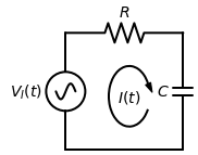
Figure 1:Circuit diagram of an RC low-pass filter.
Let denote the input voltage applied to the filter, the voltage drop across the resistor, and the output voltage, which is equal to the voltage drop across the capacitor. Using Kirchhoff’s laws, we can write:
Since the resistor and capacitor are in series, the current through them must be the same. Applying Ohm’s law to the resistor gives , and using the capacitor equation gives . Substituting these into Kirchhoff’s law equation yields:
Rearranging this, we obtain a first-order differential equation for the output voltage:
This differential equation has a general form that appears in other physical systems as well. In the next section, we rewrite it more abstractly to account for this versatility.
A Generalized Response Equation
The differential equation describing the output voltage of the RC filter circuit can be generalized to model a broader class of dynamic systems. To account for this versatility, we rewrite the equation more abstractly as:
where is a general time-varying quantity representing the state of the system, is a time-varying input or driving quantity for the system and is a system parameter that determines the response timescale. In the context of the RC filter, , , and . More generally, this equation can model any physical system whose rate of change is proportional to the difference between its current state and the input/driving quantity.
The general solution to the above equation is:
where is the initial condition. This solution encapsulates both the system’s transient response and its behavior under different input conditions .
In the next section, we examine some specific cases of interest, including the response to a constant input and a sine wave input. This builds intuition on how system response depends on input characteristics and timescale .
Solution Forms for Specific Input Cases
In this section, we examine the solution to the generalized response equation (4) for some important cases of the input . This provides insight into how the system responds under different input conditions.
Constant Input
When the input is held at a constant value, the integral term in the solution (5) evaluates to simply . Substituting this into the solution yields:
This solution describes an exponential relaxation process for the state variable . It relaxes from the initial condition towards the constant input value . The timescale for this relaxation is characterized by the rate parameter . Physically, represents how quickly the system responds to perturbations from equilibrium.
The larger the value of , the faster the relaxation occurs. In the limit of very large , the relaxation is essentially instantaneous and the state remains fixed at the input value . For smaller , it takes a longer time approaching for to settle towards .
Sinusoidal input
When the driving input takes the form of a sinusoid, such that , the solution to the generalized response equation yields additional insight. For this sinusoidal input case, the solution is:
This solution involves two competing time-dependent terms: an exponential decay governed by and an oscillatory term set by the input frequency . The relative balance of these terms depends strongly on the ratio of .
In the limit of very low input frequencies (), the decaying term becomes negligible after a transient set by , compared to the oscillatory term. Hence, closely follows the input behavior.
Conversely, for high frequencies (), it is now the oscillatory term that is negligible. In this regime, rapidly decays to zero, showing almost no response to the rapidly fluctuating driving input.
Physically, this frequency-dependent damping behavior illustrates how the intrinsic system timescale acts as a low-pass filter, smoothing out input variations that are rapid relative to . Only fluctuations with periods much longer than produce significant responses in .
General Time-Varying Input
Thus far we have considered relatively simple constant and oscillatory inputs. However, the generalized response equation is also applicable when the driving quantity exhibits more complex arbitrary time-variation.
Any continuous input defined over a finite time interval () can be represented as a Fourier series, expressing it as a sum of sinusoidal components with angular frequencies . Applying the solution derived earlier for sinusoidal inputs, the response to each Fourier component will take the appropriate sinusoidal-exponential form.
Crucially, the relative balance of decaying and oscillating terms again depends on the ratio for each frequency component . Higher frequencies satisfying will see their oscillating terms strongly attenuated according to the low-pass filtering behavior uncovered previously.
Physically, this implies the system effectively smooths and filters out rapidly fluctuating fine structure in the driving input . Only variations that are sufficiently slow, with periods much longer than the intrinsic relaxation time , produce substantive responses in the state .
Thus for a general time-dependent input, the output reflects predominantly the large-scale low-frequency properties of the input signal, stripping away higher harmonics. The parameter characterizes a sharp cutoff in the frequency spectrum separating meaningful signal from imperceptible noise.
In particular, when the characteristic timescale of the input greatly exceeds the relaxation timescale , the system achieves rapid equilibrium with respect to the slowly-evolving driving conditions. This causes the time derivative term in the generalized response equation to become negligible for times past . Consequently, the output is able to closely track the input in a quasi-steady manner, with the mathematically simplified relationship of emerging. This special case forms the theoretical basis for quasi-steady state approximations, whereby timescale separation between driving forces and system responses enables reduced representations of multi-timescale behavior through techniques leveraging the assumption of sluggish input dynamics relative to swift system adjustment.
Timescale Separation
Many natural and engineered systems exhibit dynamics governed by processes operating on separated timescales. To understand such multi-timescale systems, it is useful to employ approximations that leverage clear differences in timescale.
Consider the following prototypical 2-dimensional dynamical system:
We assume the parameter governing the dynamics is much larger than for the dynamics (). This implies that evolves much more rapidly than .
To make this timescale separation evident, we non-dimensionalize the system by rescaling time as . In the rescaled timescale, the system is:
where represents the large separation between and timescales.
This formulation, combined with the results of previous sections, suggests that will rapidly achieve quasi-steady state balance with respect to changes in the slower-varying . Specifically, for , the rate of change of () will become negligible on timescales where changes in () are observable. This allows us to make the quasi-steady state approximation that , reducing the original 2D system to a simpler 1D form governed by
Comparing Steady States and Stability of the Full and Reduced Systems
In the previous section, we derived the quasi-steady state (QSS) approximation for a prototypical two-dimensional dynamical system exhibiting timescale separation between the variables. This approximation reduced the dimensionality by eliminating the faster subsystem under the assumption that it relaxes rapidly to quasi-equilibrium.
However, for the QSS approach to be valid, the full and reduced systems should exhibit comparable qualitative behavior on long timescales driven by the slow variable(s). In this section, we test this assumption by directly comparing key properties of the full and approximated systems.
First, we analyze the reduced 1D quasi-steady state approximation given by Eq. (10). At steady state, the time derivative must equal zero, yielding the steady state condition .
To assess the stability of the system, we can perform a linear stability analysis. The Jacobian and its single eigenvalue are simply the partial derivative of the right-hand side of Eq. (10) with respect to , evaluated at the equilibrium point. That is,
Then, if , the steady state is locally asymptotically stable.
For the full 2D system, steady states satisfy both and , yielding the equilibrium conditions and . Hence, the steady state values of are the same solutions to as in the 1D reduced system.
To analyze stability, we compute the Jacobian matrix of the 2D system:
Its eigenvalues are given by:
Using the large timescale separation assumption of , we obtain the following simplified expressions for the eigenvalues—see Eq. (11):
Geometrically, this reveals that, initially, trajectories will evolve rapidly along the direction of the fast eigenvector , on a timescale of . On this transient timescale, the system approaches the slow manifold aligned with the slow eigenvector . Thereafter, with , the system dynamics are dominated by the slower motion along , characterized by the velocity given by the eigenvalue .
Although the full system displays brief two-dimensional behavior, the presence of distinctly separated timescales facilitates rapid relaxation. This allows the one-dimensional reduced approximation, which focuses solely on the slow component , to accurately describe the system’s behavior near steady states that are comparable to those of the full system. Consequently, the significant difference in timescales enables effective dimensionality reduction, justifying the analysis of the simplified one-dimensional system for gaining insights into the long-term, multi-timescale dynamics.
Discussion
In this chapter, we introduced and demonstrated the quasi-steady state (QSS) approximation technique for analyzing multi-timescale dynamical systems. By considering a generalized response equation, we developed intuition for how systems respond to different input conditions depending on their intrinsic timescale.
We then presented a prototypical two-dimensional dynamical system with separated timescales as a test case. Non-dimensionalizing time made the fast-slow behavior evident. Leveraging this timescale separation, we employed the QSS approximation to reduce the system dimensionality.
Comparing the full and reduced systems’ steady states and stability validated the approximation approach. Exploiting the assumption of wide timescale gap, we showed the conditions for stable equilibrium match between the two descriptions.
Examining the eigenstructure revealed trajectories’ initial rapid evolution along the fast eigenmode, before relaxing onto the slower manifold. Thereby, the long-term behavior reduces dimensionally to motion along this slow subsystem.
This example demonstrated how timescale separation enables analytical tractability for multi-timescale problems. By projecting dynamics onto slower variables after an initial transient, QSS approximations provide qualitative and sometimes quantitative insight into long-term behaviors of interest. Overall, this chapter established the intuition, concepts and methodology behind QSS analysis of multi-timescale dynamics.