2. Why don’t Clouds Fall? - Mathematical Modeling for Life Sciences, A Primer

Abstract

In this chapter we introduce differential equations as a tool to study change. We describe a way to classify them, and the nature of its solutions when they exist. We also introduce the concept of initial value problems to narrow down a family of solutions to a particular one, and provide a method to solve a very specific set of easily solvable differential equations. We later study a phenomenon using mathematical modeling, and show step by step the path to do so: beginning with understanding the phenomenon, to writing a mathematical expression to describe it, to solving it using the method introduced earlier in this chapter and finally to discussing the obtained results.

Introduction¶

The natural world around us is constantly changing. To adequately study and understand evolving phenomena, appropriate mathematical tools are needed to describe systems and their evolution over time. Differential equations provide just such a framework, allowing the representation of natural processes in terms of rates of change.

Specifically, differential equations relate the derivative of an unknown variable to functions of that variable and/or independent variables. For instance:

\frac{dy}{dx} = f(x),

(1)

\frac{dy}{dx} = f(x,y),

(2)

\frac{\partial y}{\partial x_1} + \frac{\partial y}{\partial x_2} = f(y, x_1, x_2).

(3)

Eqs. (1) and (2) involve a single unknown variable and are called ordinary differential equations (ODEs). Eq. (3) contains partial derivatives with respect to multiple independent variables and is thus a partial differential equation (PDE). Differential equations provide a mathematical language for quantitatively describing natural systems and how they evolve over space and time.

A solution to a differential equation refers to any function that satisfies the equation. Often, differential equations admit multiple solution functions, collectively called a family of solutions. However, real-world systems are uniquely defined by their initial state. By specifying an initial condition, the problem becomes an initial value problem. This additional information allows narrowing down the family of solutions to a single, unique solution corresponding to the system’s behavior over time. Some basic differential equations can be solved analytically through explicit mathematical techniques. But for most equations, numerical methods are necessary to approximate solutions since exact closed-form solutions are intractable.

The Method of Separation of Variables¶

Differential equations of the form $dy/dx = F(x,y)$ admit closed-form solutions via the method of separation of variables when $F(x,y)$ can be expressed as the product of a function solely of $x$ , $g(x)$ , and a function solely of $y$ , $h(y)$ :

\frac{dy}{dx} = F(x,y) = g(x)h(y).

(4)

Letting $h(y)=1/f(y)$ , Eq. (4) can be rearranged such that the variables $x$ and $y$ are isolated on opposite sides:

f(y)\frac{dy}{dx} = g(x).

(5)

This separable equation is then solved by integrating both sides with respect to $x$ :

\begin{align*} \int f(y)\frac{dy}{dx} dx &= \int g(x) dx,\\ \int f(y) dy &= \int g(x) dx, \end{align*}

(6)

provided the integrals exist.

Modeling the Fall of Cloud Droplets¶

Mathematical modeling utilizing differential equations has increasingly become a valuable complement to experimental research in understanding natural phenomena. Modeling involves more than just solving equations—it is a complete process. The first step is to develop a mathematical model through formulation of governing equations that describe the key aspects of the system or problem. Crafting an appropriate model requires balance, as models need to be sufficiently simple to analyze while still accurately representing the phenomenon. Once established, models are used to gain insights through mathematical and analytical techniques rather than just obtaining numeric solutions. Critically, the results must then be interpreted by relating the mathematical abstractions back to the real system. This contextualization provides enhanced understanding and conclusions. Moreover, answering questions through modeling often leads to new questions, thereby driving development of improved or new models in an iterative process. The overarching goal of mathematical modeling is to complement empirical studies by mechanistically linking mathematics to observed natural phenomena.

As an example of the mathematical modeling process, consider the observable phenomenon of clouds remaining suspended in the sky despite being composed of water/ice; materials denser than air. Why do clouds not simply fall to the earth under the force of gravity given the density of their constituents?

To construct an initial model to investigate this question, we begin by abstracting the intricate, large-scale cloud system into its fundamental building blocks. Clouds are formed from innumerable minuscule droplets and particulates. Therefore, modeling the dynamics of a single representative component isolates the key issue while reducing overall complexity. This abstraction enables formulation of a simplified framework to theoretically explore the forces governing a single constituent’s behavior, providing insights into the large-scale behavior of clouds as aggregates of many such parts.

At the level of the individual droplet, the key elements governing its dynamics are the downward pulling force of gravity and the counteracting upward pushing force of air resistance opposing the droplet’s movement. Other complex cloud-scale phenomena are negligible for this preliminary model. Fig. Figure 1 provides a conceptual illustration of this abstracted perspective, visually depicting the isolated droplet subject to only two delineated forces via a diagrammatic force representation.

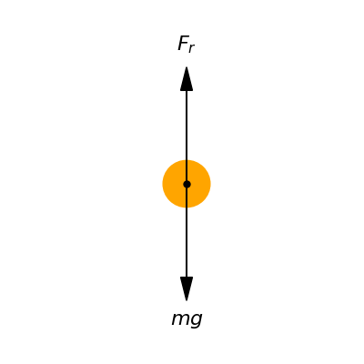
Figure 1:Diagrammatic force representation of a solitary descending water droplet (or ice particle), with the downward pointing weight and upward pointing air resistance delineated.

Consider the positive axis directed along the weight vector. Then by Newton’s second law, we can write:

ma = mg - F_r,

(7)

where $a$ is droplet acceleration, $m$ its mass, $g$ gravity, and $F_r$ frictional air force. Assuming a spherical droplet, Stokes’ law for a sphere in a fluid gives $F_r = 6\pi \mu rv$ , with $\mu$ the air viscosity, $r$ the droplet radius, and $v$ velocity. We can thus write $F_r = \eta v$ , where $\eta = 6\pi \mu r$ . Substituting into (7) and solving for $\dot{v}$ yields:

\dot{v} = \frac{\eta}{m} \left( \frac{mg}{\eta} - v \right).

(8)

Defining $\tau = m/\eta$ and $v_T = mg/\eta$ allows us to rewrite Eq. (8) as:

\dot{v} = \frac{1}{\tau} (v_T - v).

(9)

Applying the method of separation of variables to Eq. (9) yields:

\int \frac{1}{v - v_T} dv = \int \frac{-1}{\tau} dt.

(10)

Integrating both sides gives:

\ln{(v - v_T)} = \frac{-t}{\tau} + C.

(11)

Solving this for the velocity $v$ produces:

v = v_T + C e^{\frac{-t}{\tau}}.

(12)

The initial condition $v(0) = v_0$ gives:

C = v_0-v_T.

(13)

Substituting this result provides the expression:

v = v_T + (v_0 - v_T)e^{\frac{-t}{\tau}}.

(14)

Which describes the time evolution of the droplet’s velocity.

To understand the droplet’s velocity behavior over very long time periods, we calculate:

\lim_{t\to\infty} v = \lim_{t\to\infty} \left[ v_T + (v_0 - v_T) e^{\frac{-t}{\tau}}\right]= v_T.

(15)

This indicates that the droplets will eventually reach a terminal constant velocity of $v_T$ . Fig. Figure 2 displays plots of Eq. (14) for differing initial velocities $v_0$ while holding $\tau$ fixed. Notice that all solutions converge to the common value of $v_T$ , regardless of the initial conditions. This illustrates that droplets decelerate over time, eventually matching the characteristic falling speed $v_T$ defined by fluid properties and gravitational acceleration.

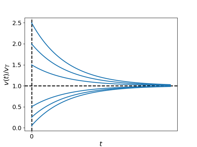
Plots of the normalized particle velocity v(t)/v_T, given by Eq. , for different initial conditions, v_0. — Figure 2:Plots of the normalized particle velocity $v(t)/v_T$ , given by Eq. (14), for different initial conditions, $v_0$ .

Let us further analyze the terminal velocity. Recall that $v_T = mg/\eta$ . However, we can express mass as $m = V\rho$ , where $V$ is droplet volume and $\rho$ its density. Since the droplet is assumed spherical, substituting gives:

v_T = \frac{V\rho g}{\eta} = \frac{\frac{4}{3}\pi r^{3} \rho g}{6 \pi \mu r} = \frac{2\rho g}{9\mu}r^{2},

(16)

which reveals the final velocity is proportional to the square of the droplet radius. That is, larger droplets reach a higher terminal speed.

Let us now explore the behavior of Eq. (14) for varying values of $\tau$ . Fig. Figure 3 displays plots of normalized particle velocity versus time for cases where $\tau/2$ , $\tau$ , and $2\tau$ are considered, while holding $v_0/v_T$ fixed. Notably, as $\tau$ increases, it takes longer for the droplet velocity to approach $v_T$ . This observation leads us to identify $\tau$ as the relaxation time of the system, representing the duration required to reach equilibrium.

To investigate the rate at which the droplet velocity approaches $v_T$ , let us examine $\tau = m/\eta$ :

\tau = \frac{m}{\eta} = \frac{V\rho}{\eta} = \frac{\frac{4}{3}\pi r^3 \rho}{6\pi\mu r} = \frac{2}{9}\frac{\rho}{\mu}r^2,

(17)

Once again, we find that $\tau$ is directly proportional to the square of the droplet radius. Therefore, larger droplets have longer relaxation times to attain their terminal velocity.

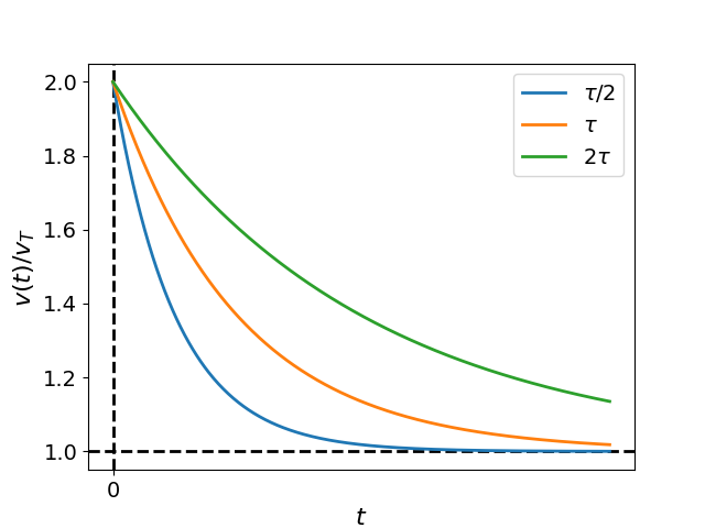
Plots of the normalized particle velocity v(t)/v_T, obtained from Eq. — Figure 3:Plots of the normalized particle velocity $v(t)/v_T$ , obtained from Eq. (14)

The above analysis provides insight into why microscopic droplets present in clouds do not readily fall under the force of gravity. Eq. (17) demonstrates that the relaxation time $\tau$ is directly proportional to the square of the droplet radius. Given typical cloud droplet sizes on the order of 10 $\mu$ m, this results in relaxation times that are exceedingly short; on the order of milliseconds based on standard fluid properties.

According to Eq. (14), these microscopic droplets would reach 99% of their terminal velocity $v_T$ within a fraction of a second due to the ultra-fast relaxation timescale. However, for cloud droplet sizes, the associated terminal velocity $v_T$ itself as given by Eq. (16) is minuscule, on the order of centimeters per second.

Therefore, over observational timescales relevant to the human eye, micrometer-sized cloud droplets do not perceptibly change in velocity. This is a result of both the very small terminal velocities and exceedingly rapid approach to equilibrium velocity. Their behavior appears static, even though they are slowly descending owing to gravity.

Only larger droplets within clouds have observable terminal velocities and thus visibly fall. Coincidentally, this analysis helps explain the triggering of rain from clouds. Precipitation occurs through coalescence of multiple microscopic droplets into larger falling raindrops, encouraged by processes like droplet collisions, updrafts/downdrafts, cooling temperatures, and presence of foreign particles.

Expanding the Model to Include Ambient Air Currents¶

Thus far, our analysis has focused on the simplified scenario where air currents are neglected and droplets fall under the isolated actions of gravity and drag forces. However, clouds exist within a dynamic atmospheric environment subjected to fluctuating air movements. To gain a more realistic perspective, let us now expand our model to include the effects of ambient wind forces.

Fig. Figure 4 displays a revised free body diagram depicting a single droplet experiencing an additional time-varying force $f(t)$ imposed by surrounding air motions. Previously, the droplet equilibrium was determined by a balance between the constant downward pull of gravity and upwards drag resistance. With inclusion of $f(t)$ , the force budget acting on each droplet becomes more complex as transient lift/drag disturbances alter the net downward acceleration at any given instant. Modeling this third force offers opportunity to deepen understanding of cloud-scale behaviors emerging from interactions between falling constituent droplets and turbulent airflow fluctuations.

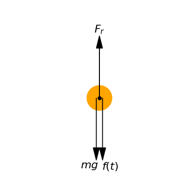
Figure 4:Free body diagram of a single falling droplet of water (or particle of ice). Pointing downwards the weight of the droplet and the force produced by an air current, and pointing upwards the resistance of the air.

Choosing the vertical axis positive in the direction of gravitational acceleration, the equation of motion is:

m\dot{v} = mg + f(t) - \eta v,

(18)

where $f(t)$ denotes the time-varying lift or drag imposed by surrounding winds. Let us define the total force acting on the droplet as $F(t) = mg + f(t)$ . Isolating the drag term in Eq. (18) yields:

\dot{v} = \frac{\eta}{m}\left(\frac{F(t)}{\eta} - v\right).

(19)

Consistent with our prior analysis, we identify the relaxation time as $\tau = m/\eta$ and the instantaneous terminal velocity as $v_T(t) = F(t)/\eta$ . Substituting these into Eq. (19) gives:

\dot{v} = \frac{1}{\tau} \left(v_T(t) - v\right) ,

(20)

which has the same form when time-varying wind effects were not included on the droplet motion.

Our previous analysis of the equation of motion without time-varying winds showed that the droplet velocity asymptotically approaches the constant terminal velocity $v_T$ , independent of initial conditions. Additionally, we determined the relaxation time $\tau$ governs how rapidly this approach occurs.

When extending our model to include time-varying winds inducing a transient terminal velocity $v_T(t)$ , similar behavior is expected for the droplet velocity $v(t)$ . Specifically, $v(t)$ will tend towards the instantaneous value of $v_T(t)$ at each moment in time. The rate at which $v(t)$ adjusts to changes in the fluctuating $v_T(t)$ is determined by the relaxation time $\tau$ .

For droplets experiencing fluctuations in $v_T(t)$ due to winds, our prior analysis indicates that those with smaller $\tau$ will track variations in $v_T(t)$ most closely over time. Within clouds, where droplet sizes yield relaxation times on the order of milliseconds, this property allows for rapid synchronization between $v(t)$ and microscale variations in airflow velocity induced by turbulence.

On observable human timescales, this near-perfect tracking imposed by minute $\tau$ obscures individual droplet motions. Instead, clouds appear nebulous and suspended motionless despite droplets smoothly adjusting their velocities downward while also following transient atmospheric currents. Therefore, the small droplet sizes characteristic of clouds effectively couple velocities to instantaneous air movements, contributing significantly to their visual appearance.

Discussion¶

In this chapter, we introduced differential equations and discussed using them to develop mathematical models of physical phenomena. We applied this approach to investigate the behavior of cloud droplets and why they do not visibly fall under gravity.

Through analytical modeling of a cloud droplet experiencing gravity, drag, and wind forces, we derived equations of motion and solved them to determine droplet velocity over time. This revealed that each droplet reaches a constant terminal settling velocity, $v_T$ , irrespective of initial conditions.

Analysis of the model showed the scaling relationships of both $v_T$ and relaxation time constant $\tau$ with droplet radius $r$ . Specifically, we found $v_T$ and $\tau$ are directly proportional to $r^2$ . Given cloud droplet radii are on the micron scale, this results in two key properties:

Droplets attain $v_T$ extremely rapidly due to exceedingly short $\tau$ .
The actual magnitude of $v_T$ is minuscule due to the $r^2$ scaling.

Therefore, while droplets gradually descend at their slow terminal velocities, this imperceptible motion occurs below human observational resolution scales.

Additionally, ambient winds disrupting continuous descent contribute further to clouds’ static visual appearance. Overall, the mathematical modeling elucidated the underlying reasons clouds evade falling visibly despite gravitational forces acting on constituent droplets.

Even simple mathematical models of natural phenomena, like the linear drag model developed here for cloud droplets, can provide deep insights into observable behaviors that may otherwise be taken for granted. By distilling relationships down to their essential mathematical elements, qualitative and quantitative predictions emerge regarding how underlying physical factors control system-level properties.

The rest of this book is dedicated to expanding on such modeling techniques, specifically through nonlinear dynamics approaches. Subsequent chapters will introduce nonlinear methods and apply them to study the time-evolving behavior of various biological systems. The overarching goal is to utilize analytical and computational nonlinear dynamics tools to elucidate the unexpectedly complex and sometimes counterintuitive dynamics that often arise in living systems due to nonlinear interactions between components.

Exercises¶

Consider an object with an initial temperature $T_0$ , a specific heat capacity $C$ , and a thermal conductance $\alpha$ . This object is placed in an oven that maintains a constant temperature $T_H$ . The rate of heat influx into the object is proportional to the difference between the oven temperature and the object’s current temperature. This relationship can be expressed mathematically as:
$J_Q = \alpha (T_H - T),$
(21)
where $T$ represents the temperature of the object at any given time. Additionally, the heat influx is related to the rate of change of the object’s temperature through the specific heat capacity $C$ :
$J_Q = C \frac{dT}{dt}.$
(22)
By combining these two equations, derive the differential equation that describes the evolution of the object’s temperature $T$ over time. After formulating the differential equation, discuss its solution in detail, focusing particularly on the concept of relaxation time, which characterizes how quickly the object approaches thermal equilibrium with the oven.
Consider an electrical circuit in which a capacitor, with capacitance $C$ , is connected to a voltage source $V_S$ through a resistor $R$ . Initially, the capacitor is uncharged, and the circuit is open. Since the resistor and capacitor are in series, the sum of the voltage drops across each component equals the source voltage:
$V_S = V_R + V_C$
(23)
Here, the current $I$ flowing through both the resistor and the capacitor is the same. According to Ohm’s Law, the voltage drop across the resistor is given by:
$V_R = I R$
(24)
Additionally, the relationship for the capacitor is described by:
$I = C \frac{d V_C}{dt}$
(25)
Taking all of this into account, derive the differential equation for the voltage across the capacitor, $V_C$ , once the circuit is closed. Identify the factors that determine the relaxation time of the circuit. Is the result intuitive?
Consider a chemical reaction in which a protein $A$ shifts forth and back between conformational states $A_1$ and $A_2$ . The forward and backward reaction velocities are:
$v_f = k_f [A_1],$
(26)
$v_b = k_b [A_2],$
(27)
with $k_f$ and $k_b$ denote the forward and backward reaction rate constants and $[X]$ represents the concentration of substance $X$ . The rates of change of $[A_1]$ and $[A_2]$ are given by:
$\frac{d[A_1]}{dt} = - \frac{d[A_2]}{dt} = - v_f + v_b .$
(28)
From these considerations and the assumption that the total concentration of $A$ molecules is constant ( $[A_1] + [A_2] = [A_T]$ ) derive a differential equation for $[A_2]$ . Study the solution and discuss how the equilibrium value and the relaxation time depend of $k_f$ and $k_b$ .
Numerically solve the differential equation
$\frac{dx}{dt} = \gamma (f(t) - x)$
(29)
for various forms of the function $f(t)$ . Specifically, consider:
- A sinusoidal function.
- A square-wave function.
- A sawtooth wave function.
Explore different values for the parameter $\gamma$ , ranging from very small to very large relative to the period of the function $f(t)$ . Plot your results and provide a discussion on the outcomes. Consider the implications of your findings for the systems analyzed in the previous exercises.