14. SIR Model - Mathematical Modeling for Life Sciences, A Primer

Abstract

The chapter introduces the fundamental SIR modeling framework, which is used to study the dynamics of infectious disease transmission. The SIR model categorizes a population into three compartments: susceptible, infected, and recovered individuals. Changes in the size of each compartment are represented by a system of differential equations, formulated based on assumptions of homogeneous mixing and exponential recovery rates. The model equations are non-dimensionalized and analyzed to identify fixed points and determine stability through Jacobian analysis. This analysis reveals a critical transition at the basic reproduction number $R_0=1$ , which governs whether a disease can invade and become established in the population. Various extensions and applications of the SIR model are also discussed, demonstrating how it can provide both qualitative and quantitative insights into real disease systems.

Introduction¶

Mathematical modeling of infectious disease transmission has been crucial for understanding and controlling epidemics. One of the simplest yet most influential epidemiological models is the SIR model. Proposed in the early 20th century, the SIR model divides a population into three categories—Susceptible, Infected, and Recovered—and represents transmission through a system of differential equations.

Despite its assumptions of homogeneous mixing and exponential recovery rates, the SIR model has provided fundamental insights into disease dynamics. Threshold quantities like the basic reproduction number $R_0$ characterize when an outbreak will occur based on transmission rates. Analytic solutions also demonstrate a range of epidemiological behaviors from disease invasion and persistence to endemic equilibrium.

The basic SIR framework has served as a starting point for extending models to consider additional biological and external influence realistically. Yet even in its simple form, the model illustrates how self-organizing transmission processes alone can lead to complex episodic outbreak patterns on the population scale. SIR analyses and simulations provide an elegant, versatile tool to study disease control strategies from targeted quarantines to vaccination programs.

In this chapter, we will introduce the SIR modeling framework in detail. We will formulate the compartmental differential equations, obtain analytic solutions, and explore simulation-based analyses. Examples will demonstrate how this basic setup can be applied to real disease systems while also motivating extensions. The goal is to establish the conceptual and technical foundations of SIR modeling as a foundation for more complex and realistic epidemiological representations.

Model Formulation¶

The SIR model divides population into three mutually exclusive compartments based on disease status: susceptible (S), infected (I), and recovered (R). The following assumptions are made:

Individuals mix homogeneously; the probability of contact between any two individuals is equal.
Upon infection, individuals immediately become infectious.
Transmission occurs through contact between susceptible and infected individuals. The rate of new infections is thus proportional to both the number of susceptible ( $S$ ) and infected ( $I$ ) individuals, with proportionality constant $\beta$ known as the transmission rate.
Infected individuals recover at a constant rate $\gamma$ and acquire lifelong immunity.
The population birth rate is constant and denoted by $\alpha$ .
Individuals in all compartments die due to causes other than disease at constant rate $\mu$ , and infected individuals also die due to causes directly associated to the disease at a constant rate $\delta$ .

Schematic representation of the SIR model compartmental structure and transitions. Susceptible individuals (compartment S) become infected at a rate proportional to contacts with infectious individuals in compartment I. Infected individuals recover at rate \gamma and enter the recovered compartment R with lasting immunity. All compartments face a baseline death rate \mu. Additionally, infectious individuals face an extra disease-induced death rate \delta owing to pathogenic effects. 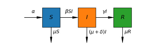— Figure 1:Schematic representation of the SIR model compartmental structure and transitions. Susceptible individuals (compartment $S$ ) become infected at a rate proportional to contacts with infectious individuals in compartment $I$ . Infected individuals recover at rate $\gamma$ and enter the recovered compartment $R$ with lasting immunity. All compartments face a baseline death rate $\mu$ . Additionally, infectious individuals face an extra disease-induced death rate $\delta$ owing to pathogenic effects.

These mechanisms are schematically represented in Fig. Figure 1 which pictures infection dynamics as flux-balance processes. Taking this into consideration, the population evolution in all compartments can then be expressed as a system of ordinary differential equations:

\begin{align*} \frac{dS}{dt} &= \alpha -\beta SI -\mu S, \\ \frac{dI}{dt} &= \beta SI - (\gamma + \mu + \delta) I, \\ \frac{dR}{dt} &= \gamma I - \mu R. \end{align*}

(1)

Normalizing the Model¶

We can non-dimensionalize the system of differential equations by introducing the following normalized variables:

\begin{align*} s &= \frac{S}{\alpha / \mu}, \\ i &= \frac{I}{\alpha / (\gamma + \mu + \delta)}, \\ r &= \frac{R}{\alpha / \mu}, \\ t'&= \mu t. \end{align*}

(2)

With this, the ODE system becomes:

\begin{align*} \frac{ds}{dt'} &= 1 - R_0 si - s, \\ \frac{di}{dt'} &= \rho (R_0 si - i), \\ \frac{dr}{dt'} &= \epsilon i - r, \\ \end{align*}

(3)

where

\begin{align*} R_0 &= \frac{\alpha \beta}{\mu(\gamma + \mu + \delta)}, \\ \rho &= \frac{\gamma + \mu + \delta}{\mu}, \\ \epsilon &= \frac{\gamma}{\gamma + \mu + \delta}. \end{align*}

(4)

The normalization process yields several advantages. First, it reduces the original model with 5 parameters to an equivalent model with only 3 non-dimensional lumped parameters. This simplifies the analysis. Second, some of these lumped parameters have special epidemiological meaning. In particular, $R_0$ is known as the basic reproductive number. To understand its significance, rewrite $R_0$ as:

R_0 = \beta \frac{\alpha}{\mu} \frac{1}{\mu+\gamma+\delta}.

(5)

$\beta$ represents the number of new infections generated by each infectious individual per unit time. $\alpha/\mu$ is the disease-free population size. Thus, $\beta \alpha / \mu$ gives the number of infections generated per unit time by one infectious individual introduced into a completely susceptible population. Meanwhile, $1/(\mu+\gamma+\delta)$ is the average time an individual spends in the infectious compartment before either recovering or dying. Multiplying these terms gives $R_0$ , which can thus be interpreted as the expected number of secondary infections produced by a single infectious individual introduced into a wholly susceptible population. The dynamical significance of this threshold will become clear in subsequent analysis.

Fixed Points and Stability Analysis¶

The first two differential equations of the normalized SIR model, governing the dynamics of $s$ and $i$ , form an autonomous subsystem that is decoupled from the equation for $r$ . This subsystem can be analyzed independently of $r$ , then the solutions for $i$ can be substituted into the third equation to solve for $r$ .

Focusing first on the independent $(s,i)$ subsystem will allow us to characterize the overall infection dynamics without consideration of the recovered population. Solving this core transmission model will provide insight into whether the disease can invade and establish infection within the population.

Rewriting this subsystem

\begin{align*} \frac{ds}{dt'} &= 1 - R_0 si - s, \\ \frac{di}{dt'} &= \rho (R_0 si - i). \end{align*}

(6)

It is straightforward to prove that it has two different fixed points:

(1,0), \quad \left( \frac{1}{R_0}, 1 - \frac{1}{R_0} \right).

(7)

To analyze the stability of the disease-free equilibrium, we compute the Jacobian matrix of the reduced subsystem:

J = \begin{bmatrix} -1 -R_0 i & -R_0 s \\ \rho R_0 i & \rho(R_0 s - 1) \end{bmatrix} .

(8)

Evaluating this at the disease-free fixed point $(1,0)$ gives:

J(1,0) = \begin{bmatrix} -1 & -R_0 \\ 0 & \rho(R_0 - 1) \end{bmatrix} .

(9)

The eigenvectors of the Jacobian matrix are:

v_1 = (1, 0), \quad v_2 = \left(-\frac{R_0}{1+\rho(R_0 - 1)}, 1\right),

(10)

with corresponding eigenvalues:

\lambda_1 = -1, \quad \lambda_2 = \rho (R_0 - 1).

(11)

These results indicate that the disease-free fixed point is locally asymptotically stable when $R_0<1$ , and unstable otherwise, transitioning to a saddle point structure at the critical value of $R_0=1$ . This stability switches at the epidemic threshold of $R_0=1$ .

We can investigate the stability of the endemic equilibrium by evaluating the Jacobian matrix at $(1/R_0, 1-1/R_0)$ :

J(1/R_0, 1-1/R_0) = \begin{bmatrix} -R_0 & -1 \\ \rho(R_0 -1) & 0 \end{bmatrix} .

(12)

Rather than computing the eigenvalues directly, which could yield cumbersome expressions, we analyze the Jacobian trace ( $\tau$ ) and determinant ( $\Delta$ ):

\tau = -R_0, \quad \Delta = \rho (R_0 -1).

(13)

From these results, we see that $\Delta<0$ when $R_0<1$ , indicating the endemic equilibrium is a saddle node in this case. Additionally, for $R_0>1$ , $\Delta>0$ and $\tau<0$ , implying that the endemic equilibrium is locally asymptotically stable. In summary, the trace and determinant criteria reveal that the endemic fixed point undergoes a transcritical bifurcation, transitioning from a saddle to a stable node as $R_0$ passes through the threshold value of 1.

Fig. Figure 2 summarizes the findings of the local stability analysis. Observe that, in the endemic state, $i^*$ takes negative values when $R_0<1$ . This means that, in practice, only the disease-free steady state exists when the average number of secondary infections produced by a single infectious individual introduced into a wholly susceptible population is less than one.

Steady-state values and stability domains as a function of the basic reproduction number, R_0. (Left) In the disease-free state, the fraction of susceptible individuals, s^*, remains at 1, represented by the blue curve. However, in the endemic-disease state s^* decreases inversely with R_0, shown by the red curve. (Right) The normalized infected fraction at equilibrium, i^*, is zero in the disease-free state (blue curve) and increases as 1 - 1/R_0 in the endemic-disease state (red curve). A transcritical bifurcation occurs at R0=1. For R0 < 1, the disease-free equilibrium is stable (solid lines) while the endemic steady state is unstable (dashed lines). At the bifurcation point, the two equilibria collide and their stability reverses for R0 > 1. 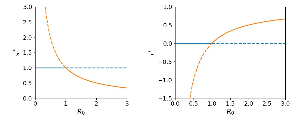— Figure 2:Steady-state values and stability domains as a function of the basic reproduction number, $R_0$ . (Left) In the disease-free state, the fraction of susceptible individuals, $s^*$ , remains at 1, represented by the blue curve. However, in the endemic-disease state $s^*$ decreases inversely with $R_0$ , shown by the red curve. (Right) The normalized infected fraction at equilibrium, $i^*$ , is zero in the disease-free state (blue curve) and increases as $1 - 1/R_0$ in the endemic-disease state (red curve). A transcritical bifurcation occurs at R0=1. For R0 < 1, the disease-free equilibrium is stable (solid lines) while the endemic steady state is unstable (dashed lines). At the bifurcation point, the two equilibria collide and their stability reverses for R0 > 1.

In summary, the SIR model predicts two possible long-term outcomes depending on the value of $R_0$ . Specifically, the model has two steady states: a disease-free equilibrium where the infection is eliminated, and an endemic equilibrium where the disease persists at a constant level in the population.

The stability analysis revealed that a critical transition occurs at $R_0=1$ . For $R_0<1$ , the disease-free state is locally asymptotically stable, meaning any small perturbation will fade out as the infection dies from the population. However, when $R_0>1$ , the disease-free equilibrium loses stability. This same threshold governs the stability of the endemic equilibrium, which undergoes a bifurcation at $R_0=1$ . Below the threshold, the endemic state is a saddle node and unstable. But for $R_0>1$ , it transitions to a stable node.

Biologically, $R_0$ represents the average number of secondary cases produced by one infected individual in a fully susceptible population. Hence, by determining whether $R_0$ is above or below one, we can predict if a disease invasion is likely to succeed or fail at establishing long-term transmission within the community. The stability analysis therefore provides key insights into disease dynamics based on the epidemiological threshold defined by $R_0$ .

Based on the definition of $R_0$ , there are a few measures that can be taken to reduce its value:

Reduce transmission rate ( $\beta$ ). Public health interventions that decrease the risk of transmission during contact, such as hand hygiene, masks, distancing, and ventilation, will lower $\beta$ . Non-pharmaceutical interventions like lockdowns and restrictions on gatherings that reduce social contact frequency also impact $\beta$ .
Increase recovery rate ( $\gamma$ ). Providing supportive medical care and targeted treatment to infected individuals can help speed their recovery and shorten the duration that they remain infectious, effectively increasing parameter $\gamma$ .
Increase removal rate ( $\delta$ ). In agricultural or wildlife settings, humane culling of visibly infected individuals can effectively increase the disease-induced mortality rate parameter $\delta$ . However, in human populations a more ethical approach is to quickly identify infectious individuals through widespread testing and rigorous contact tracing and place them in isolation.
Reduce influx into susceptible class ( $\alpha$ ). Rather than interpretation as birth rate, $\alpha$ is better viewed as the rate at which new individuals become susceptible, such as through loss of immunity. Vaccination upon birth or entrance into the susceptible population lowers this parameter without unwanted demographic effects.
Combination of approaches: The most effective strategies often combine multiple types of measures simultaneously. This creates additive reductions in $R_0$ through independent pathways compared to single measures.

Discussion¶

While the basic SIR model makes several restrictive assumptions, it has proven remarkably capable of capturing fundamental mechanisms of disease transmission dynamics. The model’s enduring value stems from its ability to isolate a minimal set of elements necessary to mathematically represent infectious propagation through a population based on transmission between individuals. Though heterogeneous mixing, temporary immunity, and other real-world complexities are ignored, the model framework provides conceptual and predictive insights that have remained highly relevant.

Despite its limitations, the SIR model elucidated critical but unintuitive properties like the existence of epidemic thresholds defined by epidemic quantities like R0. Threshold effects and bifurcation behaviors revealed through model analysis explain why certain interventions can entirely curb outbreaks while others have negligible impact. Such lessons challenge naïve assessments and guide rational intervention design.

Perhaps most remarkably, the simple SIR rules give rise to complex and varied overall infection patterns at the system scale depending on parameter conditions. Self-organized criticality and phase transition phenomena emerge from local inter-individual interactions alone. These phenomena shed light on how diseases can transition between disparate outbreak modes from fleeting invasion to endemic stability.

The model’s intrinsic value also lies in its explanatory character; by distilling phenomena to essential mathematical elements, relationships between underlying factors and observable behaviors are uncovered. This enhances conceptual understanding beyond empirical observations alone. The model serves as a framework upon which more realistic representations can be built through principled expansions, while preserving core transmission dynamics.

In summary, despite being formulated over a century ago with limited data and computational power, the SIR model has proven to transcend its restrictive assumptions through theoretical and practical insights that remain highly relevant today. Its minimal yet fundamental representation of transmission acts as the cornerstone upon which our quantitative understanding of infectious disease dynamics continues to be built.

Exercises¶

Numerically solve the SIR model using a range of parameter combinations. Be sure to verify that all parameter sets for which $R_0 > 1$ lead to steady states characterized by endemic populations of infected individuals.
Verify numerically that vaccinating at least a fraction of $1 - 1/R_0$ of newborns results in the extinction of the disease when $R_0 > 1$ . Additionally, analyze the effects of vaccinating a larger fraction of newborns.
Select parameter values such that $R_0 > 1$ and $\gamma \gg \mu$ . Numerically solve the model equations and discuss your findings.