20. The FitzHugh-Nagumo Model - Mathematical Modeling for Life Sciences, A Primer

Abstract

This chapter introduces the FitzHugh-Nagumo model, a two-variable representation of excitable dynamics. We begin by reviewing the Hodgkin-Huxley model of the neuronal action potential, which provided the first quantitative description but was too complex for broader analysis. We then motivate the need for a simplified model that could capture key properties while facilitating mathematical insights. Next, we introduce the FitzHugh-Nagumo equations and analyze their fixed points and nullclines. Through linear stability analysis and examination of phase plane portraits, we demonstrate how the system can generate self-sustained oscillations via a stable limit cycle. We show that these oscillations qualitatively reproduce the spike-and-wave behavior of excitable systems through relaxation oscillations. Finally, we discuss how the FitzHugh-Nagumo model established an important conceptual and mathematical framework for investigating fundamental principles of excitability and excitation waves in a computationally simpler setting than previous approaches.

Introduction¶

Early models of cell excitability focused on reproducing the qualitative spiking behavior of the action potential. The van der Pol oscillator provided a simple representation of self-sustained oscillations in autoexcitable systems like the heart. However, it did not account for the distinct properties of neurons and other excitable cells that require an external stimulus to trigger an action potential.

A breakthrough came with the Hodgkin-Huxley model in the 1950s. Through pioneering experimental and theoretical work, Hodgkin and Huxley developed the first quantitatively accurate model of neuronal excitation. They showed that action potentials result from non-linear interactions between voltage-gated sodium and potassium ion channels and membrane potential. This established the foundations of computational neuroscience and quantitative modeling of excitable cells.

However, the Hodgkin-Huxley model is complex, with four non-linear differential equations and multiple voltage-dependent gating variables. This complexity limited analytical insights and computation. A simpler explanatory model was needed to better understand the general principles governing excitability and oscillatory behavior in nerve and muscle fibers.

In the early 1960s, FitzHugh and Nagumo independently developed minimal two-variable models of neuronal excitability that captured the essence of excitable dynamics while removing biochemical details. These “reduced” models provided a mathematically tractable framework for analyzing properties like excitation thresholds and traveling waves.

The goal of this chapter is to introduce the FitzHugh-Nagumo model and analyze its dynamics. We will derive its equations, examine fixed points and oscillations, and discuss its applications to diverse excitable systems. The FitzHugh-Nagumo model established a new paradigm for conceptualizing excitability and remains influential for its insights into universal organizing principles of excitable media.

The Hodgkin-Huxley Model¶

The Hodgkin-Huxley model, developed in the 1950s, profoundly transformed the field of neuroscience. Prior to it, neuronal signaling was conceptualized in an oversimplified binary framework, with neurons considered to either fire an action potential or remain inactive. Hodgkin and Huxley shattered this notion by quantifying the ionic underpinnings of excitation. They established that the action potential results from finely coordinated ion movements, firmly establishing membrane biophysics as a quantitative discipline.

It is important to understand the historical context preceding this landmark achievement. In the 1930s, Cole and Curtis developed the voltage-clamp technique, permitting direct measurement of membrane ionic currents for the first time. This opened new insights into neural membrane properties. Further, Hodgkin made pioneering intracellular recordings of the action potential in squid giant axons in the late 1940s, providing new data but leaving the precise mechanisms unclear. Building on these foundations, Hodgkin joined efforts with Huxley at Cambridge University in the early 1950s. Through ingenious experimentation and quantitative modeling, they elucidated the molecular sequence of events underlying excitation. Their paired experimental and theoretical work effectively solved the mystery of how ions propagating an electrical signal across neural membranes.

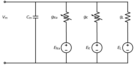
Equivalent circuit diagram of the Hodgkin-Huxley model. The membrane is represented as a capacitor separating two ionic solutions of different concentration. Conductances for sodium (g_{Na}) — Figure 1:Equivalent circuit diagram of the Hodgkin-Huxley model. The membrane is represented as a capacitor separating two ionic solutions of different concentration. Conductances for sodium ( $g_{Na}$ )

Conceptually, Hodgkin and Huxley modeled the cell membrane as a capacitor separating two ionic solutions of differing concentration: the extracellular medium and the cytoplasm. To explain ion flux dynamics, they proposed the existence of transmembrane structures, now known as ion channels, that were selectively permeable to ions like sodium and potassium. Critically, Hodgkin and Huxley hypothesized that these channels acted as variable resistors in parallel with the membrane capacitor.

Based on this ionic hypothesis, they developed the equivalent circuit diagram shown in Fig. Figure 1 to mathematically describe dynamic electric behavior in excitable cells. The governing equation for this circuit is:

I = C_M \frac{dV_M}{dt} + g_{Na} (V_M - V_{NA}) + g_{K} (V_M - V_{K}) + g_{L} (V_M - V_{L}),

(1)

where $I$ represents the total membrane current per unit area, $C_M$ is the membrane capacitance, $g_{Na}$ and $g_K$ are the sodium and potassium conductances, $V_{Na}$ and $V_K$ are the ion reversal potentials, and $g_L$ and $V_L$ characterize leak conductance and potential. The reversal potential is the membrane voltage at which net ion flow is zero. Ion flux results from electrochemical gradients comprising concentration differences and voltage potentials. At equilibrium, these counteracting forces balance and establish the reversal potential with no net ion movement. Leak currents, mediated by open leak channels permeable to ions like potassium, sodium and chloride, provide a small continuous current important for maintaining the resting potential.

In Figure Figure 1, the sodium and potassium resistors are depicted as variable to model their voltage dependence. Hodgkin and Huxley postulated that each ion channel consists of several subunits that can individually transition between open and closed conformations. They proposed that the entire channel only conducts ions when all subunits adopt the open state. To mathematically represent this, Hodgkin and Huxley defined the sodium and potassium conductances as:

\begin{align*} g_{Na} &= \bar{g}_{Na} m^3 h, \\ g_K &= \bar{g}_K n^4. \end{align*}

(2)

where $m$ , $h$ , and $n$ refer to the fraction of subunits in the open state for their respective channels. It was later discovered that voltage-gated sodium channels contain three identical subunits plus one distinct subunit, while potassium channels contain four identical subunits.

Hodgkin and Huxley modeled the dynamics of subunit conformational changes with:

\begin{align*} \frac{dm}{dt} &= \alpha_m(V_M) (1-m) - \beta_m(V_M) m, \\ \frac{dn}{dt} &= \alpha_n(V_M) (1-n) - \beta_n(V_M) n, \\ \frac{dh}{dt} &= \alpha_h(V_M) (1-h) - \beta_h(V_M) h, \end{align*}

(3)

where the transition rates $\alpha_i$ and $\beta_i$ depend on membrane potential. For brevity, we omit Hodgkin and Huxley’s specific functional forms for these rates.

Motivation for Simplification¶

While the Hodgkin-Huxley model provided the first successful quantitative description of neuronal action potentials, its complexity also limited its utility for analyzing broader dynamical properties. The model contains four nonlinear differential equations involving several voltage-dependent gating variables. This made analytical insights into its behavior difficult to obtain.

Furthermore, implementing the Hodgkin-Huxley model numerically was computationally untractable at that time due to the need to resolve fast timescales of gating variable kinetics. There was thus a need for simpler models that could retain the essential feature of excitability while facilitating mathematical analysis and simulations. The goal was to distill the Hodgkin-Huxley model down to its bare conceptual minimum in order to understand general principles governing oscillatory and excitable phenomena in nerve and muscle fibers.

This motivated FitzHugh and Nagumo in the early 1960s to independently develop simplified two-variable models of neuronal excitability that abstracted away biochemical details. While less biophysically detailed, these minimal models opened new opportunities to investigate fundamental properties like limit cycles, thresholds for excitation, and traveling wave behaviors through qualitative analysis and simulation—paving the way for novel insights into neural and cardiac dynamics.

Derivation of the FitzHugh-Nagumo Equations¶

The FitzHugh-Nagumo model was developed to capture the essential features of excitability in a simplified manner. FitzHugh drew inspiration from the van der Pol oscillator, which was known to reproduce properties of autoexcitable systems through a limit cycle behavior.

To mathematically represent neuronal excitability, FitzHugh modified the van der Pol framework such that the system’s steady state could transition between stable and unstable regimes. He proposed a two-variable formulation involving a fast membrane potential variable $V$ and slower recovery variable $R$ .

There is some flexibility in how the FitzHugh-Nagumo model is expressed mathematically. A common formulation considers the equations:

\begin{align*} \frac{dV}{dt} &= f(V) - R + I, \\ \frac{dR}{dt} &= \epsilon(\gamma V - R). \end{align*}

(4)

The function $f(V)$ represents a cubic polynomial feedback for the variable $V$ , which can take positive or negative values depending on the magnitude of $V$ . This nonlinear feedback captures the regenerative dynamics underlying excitability. In this common formulation, the nonlinear feedback is defined as:

f(V) = V (a - V) (V - b),

(5)

with $a < b$ . The small parameter $\epsilon \ll 1$ establishes a time scale separation between the fast variable $V$ and slower variable $R$ . Physiologically, this reflects the separation between rapid membrane dynamics and slower cytoplasmic processes. Due to its slower time scale, $R$ provides negative feedback to $V$ , mimicking neural recovery mechanisms that return the membrane potential to its resting level following excitation. Finally, the parameter $I$ acts as a constant input current, analogous to leak currents that determine the neuronal resting potential. Together, these features allow the FitzHugh-Nagumo model to reproduce the essential excitable spiking dynamics in a simplified mathematical framework.

Analysis of Steady States¶

To analyze the fixed points and their stability, we first find the nullclines of the system. For this system, the $V$ -nullcline corresponds to points where $\dot{V}=0$ , and the $R$ -nullcline corresponds to points where $\dot{R}=0$ . Through algebraic manipulation, these nullclines can be written as:

\begin{align*} R &= f(V) + I, \\ R &= \gamma V. \end{align*}

(6)

These nullclines are plotted in Figure Figure 2 for parameter values $a=1$ , $b=3$ , $\gamma=2.2$ , and three different values of the input current $I=0,1,2$ . We see that when $I=0,1$ , the cubic $V$ -nullcline and linear $R$ -nullcline intersect in the left branch of the cubic where $f'(V)<0$ . In contrast, when $I=2$ the nullclines intersect in the middle portion where $f'(V)>0$ .

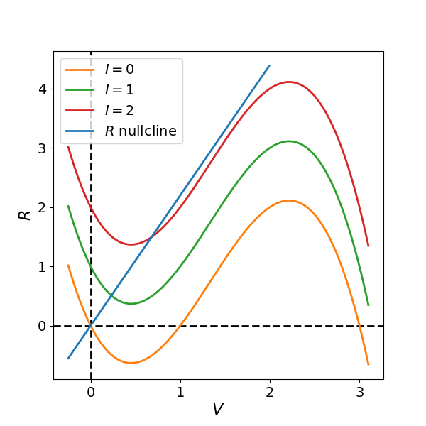
Nullcline diagrams of the FitzHugh-Nagumo system for different values of the input current I. When I=0 and I=1, the cubic V-nullcline intersects the linear R-nullcline in the left branch where f'(V)<0, yielding a stable fixed point. For I=2, the intersection occurs in the middle branch where f'(V)>0, producing an unstable fixed point. — Figure 2:Nullcline diagrams of the FitzHugh-Nagumo system for different values of the input current $I$ . When $I=0$ and $I=1$ , the cubic $V$ -nullcline intersects the linear $R$ -nullcline in the left branch where $f'(V)<0$ , yielding a stable fixed point. For $I=2$ , the intersection occurs in the middle branch where $f'(V)>0$ , producing an unstable fixed point.

Fixed points correspond to the intersections of the nullclines. To analyze their stability, we calculate the Jacobian matrix:

J = \begin{bmatrix} f'(V) & -1 \\ \epsilon \gamma & -\epsilon \end{bmatrix} .

(7)

All entries of the Jacobian are constant except for the term $f'(V)$ , which changes sign depending on whether the nullcline intersection occurs in the left or middle branch of the cubic.

The trace ( $\tau$ ) and determinant ( $\Delta$ ) of the Jacobian are:

\tau = f'(V) - \epsilon, \quad \Delta = \epsilon (\gamma - f'(V))

(8)

The stability of the system’s fixed points is governed by the sign of the Jacobian trace ( $\tau$ ) and determinant ( $\Delta$ ). By analyzing these values, we can determine how the system responds to small perturbations:

When the nullclines intersect on the outer branches of the cubic function, the trace is negative ( $\tau < 0$ ) and the determinant is positive ( $\Delta > 0$ ). This results in a locally stable fixed point, representing a neuron in its quiescent, resting state.

If the intersection occurs on the middle branch such that $f'(V) > \epsilon$ , the trace becomes positive ( $\tau > 0$ ). Under the condition $\epsilon < f'(V) < \gamma$ , the fixed point loses stability and transforms into an unstable node or spiral.

Physiologically, the parameter $\epsilon$ represents the inverse of the recovery time constant. Because the recovery variable $R$ (representing the slow gating of ion channels) evolves on a much slower timescale than the rapid membrane potential $V$ , we assume $\epsilon \ll 1$ . This separation of scales ensures that the condition for instability ( $f'(V) > \epsilon$ ) is easily satisfied once the system is pushed onto the middle branch of the cubic nullcline. This “fast-slow” architecture is what allows the model to produce the sharp, nearly vertical “jumps” in voltage that define the action potential.

Phase Plane Analysis¶

When the input current $I$ shifts the intersection of the nullclines into the middle branch of the cubic ( $f'(V) > \epsilon$ ), the fixed point becomes unstable. In the immediate vicinity of this point, the system is topologically equivalent to its linearization; because both eigenvalues of the Jacobian possess positive real parts, all trajectories in this local neighborhood flow outward.

To determine the global fate of these diverging trajectories, we apply the Poincaré-Bendixson Theorem. This theorem states that in a two-dimensional phase space, any bounded trajectory that does not approach a fixed point must asymptotically approach a periodic orbit—a limit cycle.

The existence of this limit cycle in the FitzHugh-Nagumo system can be demonstrated through three key observations:

Local Instability: The only fixed point is a repeller (an unstable node or spiral), ensuring trajectories cannot settle at equilibrium.
Global Boundedness: Far from the origin, the cubic nonlinearity $f(V)$ dominates. Large positive or negative values of $V$ result in strong restorative forces that drive the system back toward the center of the phase plane.
Absence of Singularities: The vector field is smooth and continuous across the entire $V$ - $R$ plane, with no other fixed points to “trap” the flow.

As shown in Fig. Figure 3, any trajectory starting near the unstable fixed point spirals outward, while any trajectory starting very far away is pushed inward: they first converge to the $V$ -nullcline to then approach the fixed point following the nullcline. Consequently, the flow is “trapped” within a compact region of the phase plane. Because it cannot escape to infinity and cannot return to the repelling fixed point, it must settle into a unique, stable limit cycle. This periodic orbit is the mathematical manifestation of the continuous, repetitive “spiking” observed in autoexcitable cells.

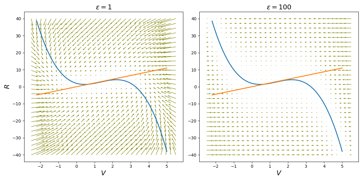
Phase portraits of the FitzHugh-Nagumo oscillator for parameter values a=1, b=3, \gamma=2, and 2 different values of parameter \epsilon, overlaid with nullclines. Arrows indicate vector field flow. — Figure 3:Phase portraits of the FitzHugh-Nagumo oscillator for parameter values $a=1$ , $b=3$ , $\gamma=2$ , and 2 different values of parameter $\epsilon$ , overlaid with nullclines. Arrows indicate vector field flow.

Relaxation oscillator behavior¶

When the parameter $\epsilon$ governing the time scale of the recovery variable $R$ is very small ( $\epsilon \ll 1$ ), the FitzHugh-Nagumo model exhibits relaxation oscillation dynamics. In the phase plane (Fig. Figure 4), the intersection of the nullclines occurs on the middle branch of the cubic $V$ -nullcline. Here, the local geometry and the separation of time scales render the fixed point unstable, trapping the system’s trajectories within a high-amplitude stable limit cycle.

The limit cycle is characterized by a distinct alternation between “fast” horizontal jumps and “slow” vertical drifts:

The Fast Excitation (Spike): When the system is slightly to the left of the $V$ -nullcline’s left branch, the vector field points sharply to the right. Because $V$ is the fast variable, the trajectory “jumps” horizontally across the phase plane to the right branch. This rapid transition represents the depolarization phase of the action potential.
The Slow Refractory Drift: Once on the right branch, the trajectory is forced to crawl upward along the curve. Since $\epsilon$ is small, the recovery variable $R$ increases slowly. This represents the plateau or peak of the action potential.
The Fast Repolarization: Upon reaching the local maximum (the “knee”) of the cubic nullcline, the trajectory can no longer stay on the right branch. It jumps horizontally back to the left, representing rapid repolarization.
The Slow Recovery: Finally, the trajectory drifts slowly downward along the left branch as $R$ decreases, representing the refractory period.

Consequently, the limit cycle trajectory is composed of rapid horizontal excursions and slow vertical crawls. This behavior is the mathematical basis for the periodic firing seen in autoexcitable systems, such as cardiac pacemaker cells and rhythmic neurons.

Phase portrait for \gamma\ll 1 illustrating relaxation oscillations. Thick green lines trace the limit cycle trajectory, rapidly switching between lateral branches of the V-nullcline at local minima/maxima and slowly creeping along branches. Arrows indicate vector field flow. During rapid excursions, the membrane potential spikes, while the slower recovery variable R modulates the falling and rising phases. 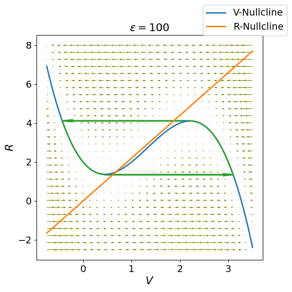— Figure 4:Phase portrait for $\gamma\ll 1$ illustrating relaxation oscillations. Thick green lines trace the limit cycle trajectory, rapidly switching between lateral branches of the $V$ -nullcline at local minima/maxima and slowly creeping along branches. Arrows indicate vector field flow. During rapid excursions, the membrane potential spikes, while the slower recovery variable $R$ modulates the falling and rising phases.

Applications to Excitable Systems¶

While initially developed as a simplified model of neuronal action potentials, the FitzHugh-Nagumo model is universal in its ability to reproduce the core properties of excitable and autoexcitable systems. Through variations in its parameter values, it can replicate important behaviors observed experimentally across diverse excitable cell and medium types.

In neurons, changes in the applied current $I$ allow the model to transition between quiescence at low $I$ and repetitive spiking at higher $I$ above a threshold, closely mimicking rheobase properties. Varying the recovery time scale $\epsilon$ alters spike frequencies, qualitative matching adaptation properties seen in neuronal firing patterns.

In cardiac tissue, decreasing $\epsilon$ slows oscillation periods, akin to effects of slowing heart rates via vagus nerve stimulation. Altering excitability parameters $a,b$ reproduces changes in action potential shape seen with altered ion channel expression levels. Propagating wavefronts of activity in the two-dimensional FitzHugh-Nagumo model with spacial coupling emulate cardiac conduction.

Even in non-biological chemical and physical systems, the model applies. Light-sensitive Belousov-Zhabotinsky reactions and lipid bilayers are autoexcitable, supported by the phase plane framework through a supercritical Andronov-Hopf bifurcation as a control parameter is varied. Self-igniting flames and autocatalytic surface reactions behave as subexcitable media between quiescent and oscillatory phases.

Overall, the FitzHugh-Nagumo equations provide a versatile mathematical description illuminating universal organizing principles for excitability. Its canonical form enables reduced computational requirements compared to detailed biophysical models while still faithfully reproducing qualitative phenomena across media exhibiting rapid switching between stable steady states. This makes it a mainstay for investigating general properties of excitability and excitation wave propagation.

Discussion¶

In this chapter, we introduced the FitzHugh-Nagumo model as a simplified two-variable representation of neuronal excitability. While far more abstract than the original Hodgkin-Huxley formulation, the FitzHugh-Nagumo model effectively distills the essential features of excitable dynamics down to their conceptual minimum.

Through its formulation as a fast-slow system with a cubic nonlinearity and recovery variable, the FitzHugh-Nagumo model can reproduce the hallmark electrical spiking behavior of neurons in a qualitatively accurate manner. Analysis of its nullclines and fixed point stability provided insight into how subthreshold oscillations arise via a supercritical Andronov-Hopf bifurcation.

Examination of the model’s phase plane portraits and vector field flows demonstrated its ability to generate relaxation oscillations, closely mimicking the characteristic spike-and-wave profile of excitable membranes. This oscillatory behavior emerges from a stable limit cycle attracted to when the fixed point loses stability.

Importantly, simulations and applications to diverse excitable media indicated the FitzHugh-Nagumo model captures universal organizing principles, not just details specific to neurons. It provides a computationally simpler framework than biophysical models while still faithfully replicating qualitative excitable phenomena.

Overall, the FitzHugh-Nagumo equations established a new paradigm for conceptualizing and mathematically investigating excitability. Their development illuminated fundamental properties of excitable systems and excitation wave propagation in a more tractable setting than earlier approaches. This makes the FitzHugh-Nagumo model highly influential as a foundational tool for studying excitation across many fields.

Exercises¶

Numerically solve the Fitzhugh-Nagumo model and plot the solutions in the phase plane, including the system’s nullclines. Explore various parameter sets and confirm that the behavior aligns with that of excitable cells when the fixed point is stable and $\epsilon \gg 0$ . Specifically, demonstrate that an action potential occurs whenever the initial condition lies to the right of the middle branch of the cubic nullcline.
A phase response curve (PRC) is a tool used to analyze the timing of action potentials in oscillatory systems. It describes how the timing of a subsequent spike is affected by perturbations (e.g., small inputs) at different phases of the oscillation cycle. In this exercise, you will compute and plot the phase response curve for the Fitzhugh-Nagumo model under parameters that cause it to behave as a relaxation oscillator. Instructions:
1. Set Up the Fitzhugh-Nagumo Model. Choose parameters such that the system exhibits relaxation oscillations.
2. Numerically solve the system using appropriate initial conditions to generate a limit cycle.
3. Apply small perturbations to the system at various phases of the oscillation. For example, modify $x$ by a small amount $\delta$ at different points in the cycle.
4. For each perturbation, measure the resulting phase shift of the next action potential. This can be done by observing the time until the next spike occurs.
5. Plot the phase shifts against the phase of the oscillation at which the perturbations were applied. The x-axis should represent the phase of the cycle (ranging from 0 to 1), and the y-axis should represent the corresponding phase shifts.
6. Discuss the characteristics of the phase response curve. Identify regions of phase advance and delay and relate them to the dynamics of the Fitzhugh-Nagumo model.