Abstract
This chapter explores the logistic growth model, a cornerstone of theoretical ecology that introduces density-dependent feedback to resolve the physical limitations of exponential expansion. Beginning with the historical transition from Malthus’s conceptual warnings on resource scarcity to Verhulst’s first quantitative formulation, we derive the logistic differential equation and its explicit closed-form solution. We demonstrate that the model’s hallmark is its long-term convergence to a stable carrying capacity (), a global attractor independent of initial population size. Through a dual approach of local stability analysis and graphical methods, we characterize the system’s fixed points and classify the resulting growth trajectories—identifying the transition from sigmoidal (S-shaped) curves to monotonic convergence. By distilling complex ecological constraints into a parsimonious mathematical framework, the logistic model serves as a fundamental pedagogical tool for understanding how nonlinear feedbacks govern the stability and regulation of real-world biological populations.
Introduction
While the exponential growth model provides a simple and mathematically tractable framework for studying populations over short time periods, it has significant limitations when extrapolated over long timescales. Most notably, the model predicts unconstrained population expansion leading to infinite size, which is not feasible in reality. All natural populations are bound by finite resources in their environment. The exponential model also ignores factors like resource competition and carrying capacity effects that act to slow growth as the population approaches the limits of its habitat. As a result, the model cannot realistically depict long-term population behavior or stability. For populations existing in a closed ecological system with density-dependent influences, another type of population model is needed that incorporates limitations on growth from resource limitations and crowding effects. This will allow an investigation of population regulation and equilibrium conditions. The development of such a model, which involves including density-dependent feedback in the growth term, is necessary to more accurately represent population dynamics over long periods aligned with biological timescales.
A Brief Historical Review
Thomas Malthus was one of the earliest scholars to study population dynamics. In his 1798 treatise An Essay on the Principle of Population, Malthus hypothesized that human populations have an inherent capacity to grow exponentially if unchecked by outside forces. This is because populations can increase geometrically through reproduction. In contrast, he argued that the food resources required to support growing populations only increase in an arithmetic progression over time. As populations grow exponentially yet resources increase linearly, Malthus recognized that individuals would inevitably come into competition for limiting resources like food, space, and other necessities of life. This competition, he proposed, serves to slow population growth from its unchecked exponential rate down to a level sustainable given the available resources. Malthus’ ideas introduced the concept that populations are regulated by external factors related to resource availability and by the scarcity and struggle for existence that arises due to overpopulation. His insights formed the basis for later formal mathematical models of population dynamics.
While Malthus recognized that populations cannot grow exponentially indefinitely, he did not provide a mathematical model to describe how growth becomes limited over time. It was the Belgian mathematician Pierre Verhulst who first developed an explicit equation incorporating this regulation mechanism. In 1838, Verhulst modified the simple exponential growth model based on Malthus’ arguments about competition for resources. He proposed adding a negative feedback term that increases in proportion to the population size, representing the growing scarcity and resultant effect on per capita growth rate as the population approaches the environment’s carrying capacity.
The Logistic Model
We begin by recalling the differential equation that governs exponential population growth:
where is a constant growth rate parameter. Verhulst proposed modifying this model by substituting parameter with a decreasing function of the population size , denoted . Specifically, he proposed a linear decay function of the form:
where represents the intrinsic per capita growth rate in the absence of density-dependent effects. Meanwhile, denotes the environment’s biological carrying capacity; the maximum sustainable population size given resource constraints. This negative feedback term grows proportionally as approaches , introducing density-dependent regulation into the exponential growth formulation. Verhulst’s ingenious substitution of a variable growth rate function was a landmark development that produced the first quantitative model embodying Malthus’ concept of self-limitation through resource competition.
Through this modification, Verhulst produced the following nonlinear ordinary differential equation to govern population dynamics:
Verhulst named the solution to this differential equation the “logistic function”. By extension, the overall model is commonly referred to as the “logistic model” of population growth. However, it is also appropriately termed the “Verhulst model”
We can solve the logistic differential equation—Eq. (3)—using variable transformations. First, introduce the change of variable . This transforms Eq. (3) to:
Next, define the variable , yielding:
This has the solution , where is the initial value. Transforming back through the steps, we arrive at the solution for the original variable :
Through judicious variable substitutions, we have derived an explicit closed-form solution to the logistic differential equation governing population dynamics.
Eq. (6) is the well known logistic function. Consider the characteristics of this solution. The first term inside the brackets, , represents the asymptotic carrying capacity. As time increases, the exponential term monotonically decays to zero. Therefore, in the limit of large time, the population will approach the value:
This shows that regardless of the initial population , the solution will always converge to the environmental carrying capacity . Physically, this makes sense; as time progresses, density-dependent effects will gradually dampen the growth rate until it balances perfectly with mortality to establish an equilibrium at the maximum sustainable size. The timescale to reach this steady state depends on the intrinsic growth rate , but the ultimate attractor is always . Therefore, the logistic model comprehensively captures the self-regulation of populations towards their local resource limits envisioned by Malthus.
Local Stability of Steady States
While we derived an analytical solution for the logistic equation in the previous section, such closed-form expressions are rare for more complex nonlinear systems. However, even when an exact solution is unattainable, we can extract profound qualitative insights by examining the system’s steady states and their local stability. While analytical solutions provide a specific map of trajectories over time, stability analysis offers a rigorous framework for predicting long-term behavior. In this section, we adopt this perspective—identifying the logistic model’s fixed points and applying linearization to determine whether the system naturally recovers from, or diverges after, small perturbations.
To perform a local stability analysis, we first express the logistic differential equation—Eq. (3)—in the general autonomous form:
where the growth rate function is defined as:
The steady states (or fixed points) of the system occur where the rate of change is zero (). Setting the growth function to zero and solving for yields two distinct fixed points:
: The trivial equilibrium (extinction).
: The non-trivial equilibrium (carrying capacity).
The stability of these points is determined by the linearization of the system. We calculate the derivative of to determine the slope of the growth function at each equilibrium:
By evaluating this derivative at each fixed point, we can classify their stability based on the sign of the result (assuming ).
At :
Because , the slope is positive. This indicates that small perturbations will grow exponentially away from zero, making an unstable fixed point.
At :
Because , the slope is negative. This indicates that small perturbations will decay over time as the population returns to equilibrium, making a locally stable fixed point.
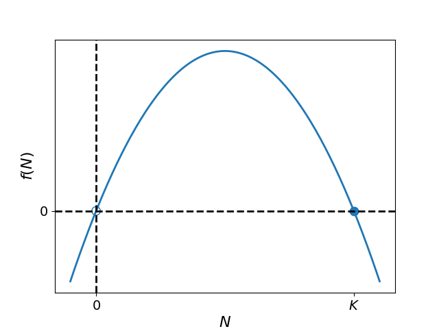
Figure 1:Graphical analysis of fixed points and stability in the logistic growth model. This figure shows the growth rate function . The two roots of this function, where it intersects the horizontal axis, are the fixed points (steady state solutions): and . Local stability is determined by the slope of at each fixed point. At , the slope is positive indicating nearby trajectories will diverge over time. Therefore, denotes an unstable fixed point, represented by an open circle. In contrast, the slope of is negative at the carrying capacity . Thus, small perturbations will contract back towards the fixed point. This characterizes as a stable steady state solution, shown as a filled circle.
The analytical results can be interpreted geometrically by examining the graph of the growth rate function, . As shown in Fig. Figure 1, the fixed points and are the roots where the parabola intersects the horizontal axis.
In this graphical framework, local stability is determined by the sign of the function on either side of a fixed point. At , the function is positive for small , indicating that the population will increase and move away from the origin; thus, is an unstable node (represented by an open circle). Conversely, at the carrying capacity , the function is positive for and negative for . This ensures that trajectories from both directions converge toward , characterizing it as a locally stable steady state (represented by a filled circle).
Beyond stability, this graphical analysis reveals the qualitative “shape” of the population’s path. Because is a concave-down parabola with a peak at , we can predict two distinct growth behaviors:
Sigmoidal Growth (): If a population starts below half the carrying capacity, it enters a region where the growth rate is increasing (). It accelerates until it hits the midpoint , after which the rate begins to decrease (), resulting in the characteristic S-shaped sigmoid curve.
Decelerating Convergence (): For populations starting above the midpoint, the growth rate is already in decline. These populations decelerate immediately as they approach . If , the growth rate is negative, and the population declines monotonically toward the carrying capacity.
By examining the slope and curvature of , we can thus predict the inflection points and long-term fates of the system without ever solving the differential equation.
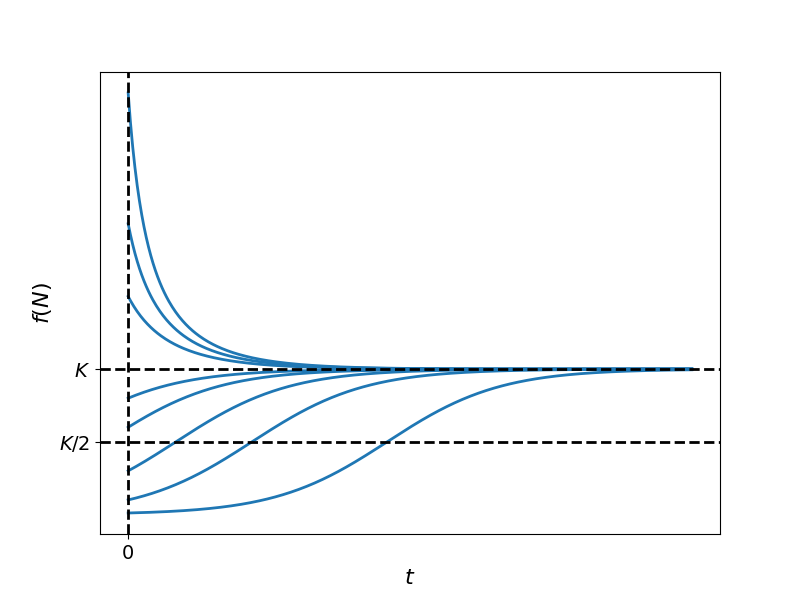
Figure 2:Qualitative trajectories of the logistic solution for varying initial conditions. This figure graphically depicts the logistic function given by Eq. {eq}`eq:08.02
The qualitative insights derived from the growth rate function, , are directly reflected in the time-dependent behavior of the system. By plotting the analytical solution—Eq. {eq}eq:08.02—over time for various initial conditions , we can visualize the emergent dynamics of the model (Fig. {ref}fig:08.02). For populations initialized below half the carrying capacity (), the trajectories exhibit an inflection point at , resulting in the classic sigmoidal (S-shaped) growth curve. Conversely, for initial conditions above this threshold (), the growth rate is strictly decreasing, leading to monotonic convergence toward the carrying capacity .
Discussion
The logistic equation, despite its minimalist structure, captures the essential mechanics of real-world population dynamics. By introducing a nonlinear, density-dependent feedback loop, the model mathematically simulates the physical constraints of finite resources and intraspecific competition. This results in the carrying capacity behavior observed across nearly all biological scales—from the proliferation of microbial colonies in a petri dish to the stabilization of ungulate populations in the wild. The model’s enduring success in mathematical biology stems from its ability to distill complex ecological pressures into fundamental processes, offering a universal baseline for understanding population outbreaks, collapses, and eventual stabilization.
Exercises
Find the steady states of the following variation of the logistic model:
Analyze the stability of these steady states and discuss the implications of your findings in comparison to the behavior of the original logistic model. Consider how the additional term affects population dynamics and equilibrium points.
Consider the following differential equation . Find all the fixed points and classify their stability. Sketch the plot of x(t) for various initial conditions.
The growth of cancerous tumors can be modeled by the Gompertz law: , where is proportional to the number of cells in the tumor, while are model parameters. Find the steady state and classify their stability. Interpret and biologically. Sketch the plots of for various initial conditions.