Abstract
This chapter introduces the canonical second-order differential equation governing damped harmonic motion as one of the most fundamental and ubiquitous models for describing oscillatory behavior near equilibrium across physics, engineering, and biology. The governing equation is derived from first principles using physical analogs including a spring-mass system, pendulum, and RLC electrical circuit. Analytical solutions to the differential equation are explored and qualitative analysis of its dynamics is performed by reformulating it as a system of first-order equations, characterizing stability properties through eigenvalue analysis and classifying oscillatory regimes. Overall, the chapter establishes the broad relevance of the damped harmonic oscillator framework while providing context for future examination of oscillatory phenomena through dynamical systems theory.
Introduction
The harmonic oscillator is one of the most ubiquitous models found across physics, engineering, and biology. At its simplest, a harmonic oscillator describes the oscillatory motion of a mass attached to an ideal linear spring. Due to the restoring force exerted by the spring in response to displacement from equilibrium, the motion takes the form of simple harmonic oscillations.
More generally, any physical system that displays oscillatory behavior about an equilibrium point can be approximated as a harmonic oscillator, provided the restoring force is proportional to displacement and acts in the opposite direction. Examples include the vibrations of molecules, pendulums with small amplitude swings, electrical circuits containing inductors and capacitors, and even whole organs or organisms displaying rhythmic dynamics like the beating of the heart or circadian rhythms.
In reality, no oscillator is truly isolated from its environment. Damping forces arising from friction or dissipation act to sap the oscillator’s energy over time. This gives rise to the damped harmonic oscillator model, where a force proportional but opposed to velocity is included. The damped harmonic oscillator provides a minimal yet remarkably versatile modeling framework applicable across science and engineering.
In this chapter, we introduce the damped harmonic oscillator differential equation from three physical perspectives: a mass-spring system, a pendulum, and an electrical RLC circuit. Through linearization and stability analysis techniques, we explore the oscillator’s steady state behavior and classify different regimes of underdamped, critically damped, and overdamped motion. Finally, we discuss examples of biological oscillators that adhere to damped harmonic dynamics, establishing the broad relevance and fundamental importance of this ubiquitous model.
Spring-mass system
We begin our examination of the damped harmonic oscillator by considering the classical spring-mass system. As shown in Fig. Figure 1, this consists of a point mass attached to an ideal linear spring with stiffness constant . The spring exerts a restoring force proportional to the displacement of the mass from its equilibrium position, according to Hooke’s law: .
In addition to the conservative restoring force of the spring, the system experiences a dampening force due to friction as the mass oscillates. We model this as a viscous drag force proportional to velocity: , where is the damping coefficient.
By Newton’s second law, the equation of motion for this system is given by:
By scaling time by , the equation takes the form:
where the damping ratio characterizes the relative contribution of damping forces.
This spring-mass representation provides a straightforward mechanical depiction of the damped harmonic oscillator and will serve as a useful reference point for discussion. The normalized equation governs a wide range of oscillatory systems, as we will explore in subsequent sections.
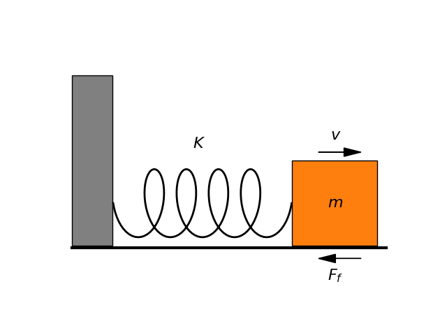
Figure 1:Spring-mass system with friction.
Pendulum
We next consider how the damped harmonic oscillator model applies to small oscillations of a physical pendulum. As illustrated in Fig. Figure 2, this consists of a point mass hanging from a rigid rod of length , which is fixed at one end to a pivot.
For small angular displacements from the hanging equilibrium position, the gravitational torque on the mass can be approximated as . Additionally, the pivot exerts a viscous damping torque opposing the angular velocity.
Treating the mass-rod system as a rigid body with moment of inertia , Newton’s second law for rotational motion gives:
where is the angular acceleration. This yields the equation of motion:
Non-dimensionalizing via the rescaling , we obtain the normalized form of the damped harmonic oscillator with damping ratio :
Thus, despite involving circular rather than linear motion, the mathematical description of small oscillations in a simple pendulum is identical to that of the spring-mass system. Both phenomena are governed by the ubiquitous damping harmonic oscillator equation near their equilibrium points.
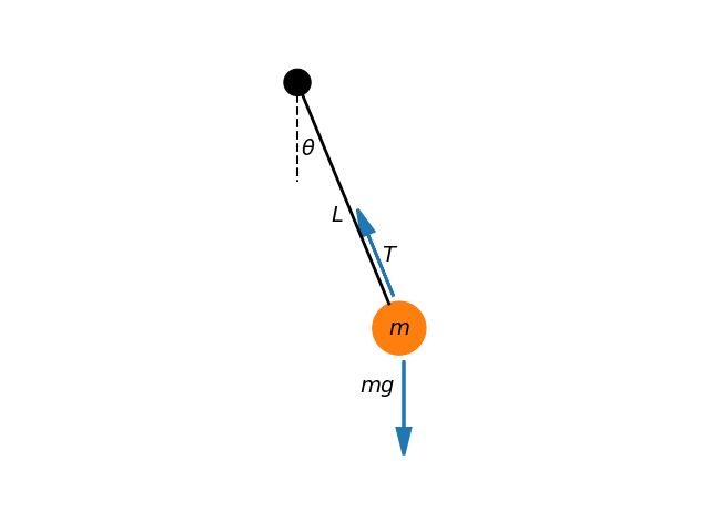
Figure 2:Pendulum displaying small angular displacement .
RLC Circuit
We now show that oscillatory behavior in an electrical RLC circuit is also described by the damped harmonic oscillator model. Consider the series circuit in Fig. Figure 3 consisting of a resistor , inductor , and capacitor .
Using Kirchhoff’s voltage law around the closed loop, we write:
where is the current through the inductor. The first term accounts for the back electromotive force induced in the inductor according to Faraday’s law. The second term represents resistive voltage drop from Ohm’s law. The final term incorporates the voltage accumulated across the capacitor from charge integration.
Taking the time derivative and rearranging yields the governing differential equation:
Upon non-dimensionalizing time as and defining the damping ratio , we obtain the normalized damped harmonic oscillator equation:
Thus, oscillations in the RLC circuit are mathematically equivalent to those in the spring-mass and pendulum systems near equilibrium. Despite physical differences, the key attribute shared is oscillatory dynamics governed by a second-order differential equation with damping. This establishes a fundamental systems-level correspondence that will prove insightful moving forward in analyzing oscillatory phenomena across diverse domains.
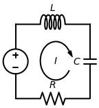
Figure 3:RLC series circuit.
Steady State Analysis
We can gain further insights by recasting the damped harmonic oscillator equation as a system of first-order differential equations. Starting from the second-order form:
Define a new variable to represent velocity. This allows us to write the original equation as a coupled system:
In vector form:
where while the Jacobian matrix is:
Due to the linearity of the system, it possesses a single fixed point given by the zero vector, . We can determine the general solution by exploiting the eigenstructure of the Jacobian matrix . Specifically, the eigenvalues and corresponding eigenvectors of allow us to write the solution as:
with and arbitrary constants determined by the initial conditions.
The eigenvalues of the Jacobian matrix at the origin are:
For a damping ratio of , the eigenvalues are purely imaginary, indicating that the fixed point is a center. When , the eigenvalues form a complex conjugate pair with negative real parts. Therefore, the fixed point is a stable spiral; perturbations will result in damped oscillations converging towards the steady state. This regime corresponds to underdamped oscillations. Finally, for , the eigenvalues are both real and negative. In this case, the fixed point is a stable node; perturbations decay monotonically without oscillation. The system is said to be in the overdamped regime.
In closing, we note that the only means of achieving truly undamped oscillations with would be in an idealized, isolated system without any dissipative effects. However, the second law of thermodynamics dictates that all real physical systems experience some form of damping or energy loss over time. The damping terms in our analysis have accounted for these non-conservative effects that cause oscillatory motions to gradually lose energy and amplitude. The type of decay—overdamped, critically damped, or underdamped oscillations—depends sensitively on the relative strength of damping represented by the dimensionless ratio .
Application to Biological Systems
Many fundamental biological processes exhibit oscillatory dynamics that can be modeled as damped harmonic oscillators. Some key examples include:
Muscle contraction/relaxation: The cyclic interaction of actin and myosin filaments, driven by ATP hydrolysis, gives rise to damped oscillations. The viscoelastic properties of muscle fibers introduce damping.
Neural oscillations: Large populations of neurons can fluctuate collectively near a limit cycle regime. Damping regulates transitions between distinct firing states.
Cardiovascular system: Each heartbeat and respiratory cycle involves pressure and volume oscillations that are smoothed by viscous damping into pressure-volume loops.
Gene regulation: Negative feedback in transcription/translation causes gene expression levels to oscillate. Molecular noise and resource depletion attenuate the oscillations over time.
While real biological systems are high-dimensional and stochastic, damped oscillator theory provides qualitative insights into self-sustained rhythms, resonance effects, and characteristic relaxation timescales. For instance, analysis of damping ratios could inform drug delivery strategies that modulate the rate at which oscillations decay.
However, the damped harmonic oscillator has limitations in describing some biological oscillators. In particular, relaxation oscillators may better capture the repetitive behavior of autoregulated cells like cardiac pacemaker cells. Relaxation oscillators exhibit alternating periods of stasis and rapid switching between states, resembling a staircase waveform arising from thresholds in the system dynamics. In the next section, we analyze relaxation oscillators to understand the core properties underlying rhythmic behaviors in tissues such as the heart.
Discussion
In this chapter, we explored the damped harmonic oscillator model; a fundamental oscillatory system found throughout physics and biology. We derived the canonical second-order differential equation that governs damped harmonic oscillations and analyzed its properties both analytically and qualitatively.
We also showed how real-world phenomena involving oscillatory motion in springs, pendulums, and electrical circuits can often be approximated as damped harmonic oscillators. This revealed the broad applicability and insights provided by studying these foundational systems.
However, damped harmonic oscillator have some limitations in capturing certain biological oscillators. In particular, relaxation oscillators may better describe the behavior of excitable cells like cardiac pacemaker cells that exhibit an alternating staircase-like waveform.
This sets the stage for the next chapter, where we will introduce and analyze relaxation oscillators. Characterizing these self-sustained oscillating systems will advance our quantitative and mechanistic understanding of rhythmic processes in living tissues and their relationship to cellular-level properties of excitability and threshold dynamics.
The overarching goal of examining damped and relaxation oscillators is to build dynamical system models that provide conceptual links between distinct realms which, at the component level, may seem very different but share underlying mathematical commonalities at a system-wide scale.
Exercises
Numerically solve the differential equation
for various values of the parameter , both above and below the critically damped regime (). Consider the initial conditions , . Plot the solutions of versus . Identify the value of that results in the fastest decay and explain the underlying reasons for this behavior.
Numerically solve the differential equation from the previous exercise with the initial condition and various values of , both positive and negative. Plot the solutions of versus . Next, repeat the exercise for increasing values of the parameter . Discuss the behavior of the solutions in the regime where . Additionally, compare these results with the solutions of the differential equation
with the initial condition , which yields
Reflect on your observations.