Abstract
Oscillatory phenomena are ubiquitous in nature and underlie diverse biological and physical processes. The van der Pol oscillator introduced by Balthasar van der Pol in 1926 established a seminal mathematical framework for describing self-sustained oscillations that arise via a distinctive relaxation mechanism. This chapter analyzes the dynamical properties of the van der Pol oscillator through analytical and qualitative techniques. We derive the governing equation of motion from first principles using a spring-mass analog and examine its behavior both near and far from equilibrium. Through linearization and phase plane analysis, we classify oscillation regimes and determine stability properties of steady states. We also relate the system’s dynamics to physiologically relevant relaxation oscillations in excitable media like cardiac tissue. Overall, the chapter establishes the van der Pol oscillator as a foundational model exhibiting nonlinear relaxation phenomena of widespread relevance across science and engineering disciplines.
Introduction
Oscillators have widespread applications in science and engineering. In the early 20th century, the field of telecommunications faced the challenge of developing self-sustained oscillators capable of powering wireless communication over long distances. Pioneering researchers experimented with resistor-capacitor-inductor (RCL) circuits and introduced amplifiers to counteract energy losses and enable sustained oscillations. However, a more rigorous understanding of these oscillator systems was needed to facilitate their further development and practical applications.
In 1926, the Dutch physicist Balthasar van der Pol made seminal progress in this area with his oscillator model. Van der Pol recognized that amplifiers behave as negative resistors at low oscillation amplitudes, effectively amplifying signals. In an ideal system, an amplifier could then induce ever-growing oscillations by substituting the resistor in an RCL circuit. However, van der Pol also realized that unbounded growth was not observed in practice, suggesting the presence of a mechanism curtailing growth.
To address this, van der Pol introduced a model term that mimicked an amplifier at low amplitudes but behaved like a resistor at high amplitudes, limiting oscillation growth. Through analyzing this model, van der Pol demonstrated that under certain parameters, self-sustained oscillations could arise via a distinctive “relaxation-type” behavior. This conceptualization of relaxation oscillations was highly influential.
Importantly, van der Pol also recognized the relevance of his model to describing the rhythmic electrical activity underlying cardiac pacemaker cells. He developed related models to simulate cardiac arrhythmias, providing novel insights.
In this chapter, we will explore the oscillatory dynamics of van der Pol’s system. Studying this model aims to deepen understanding of engineered and biological self-oscillators exhibiting relaxation phenomena.
The van der Pol model
To build his model, van der Pol substituted the linear damping term in the harmonic oscillator equation with a nonlinear term, as follows:
The key feature of this model is the nonlinear term , which mimics the behavior of an amplifier at low amplitudes (when ) but acts like a resistor at high amplitudes (when ). The parameter controls the strength of the nonlinear damping. When , the system reduces to the standard harmonic oscillator. However, for nonzero , the nonlinear damping term gives rise to richer dynamical behavior that will be explored in later sections. Specifically, as increases, the system exhibits oscillations that converge to a stable, finite-amplitude closed orbit called a limit cycle.
It is insightful to rewrite the model as a system of first-order differential equations. Here, we apply the Liénard transformation , which yields:
This formulation enables analysis techniques like phase plane analysis, which provide insight into the limit cycle behavior. Specifically, we can examine the nullclines and flow field to understand how oscillations converge to the stable limit cycle trajectory.
Steady State and Stability Analysis
To analyze the dynamics of the van der Pol oscillator, we first investigate its steady state behavior (recall that at the steady state, both derivatives and are equal to zero). It is insightful to examine the concept of nullclines in this analysis. A nullcline is defined as the set of points where one of the time derivatives is equal to zero, while the other is allowed to vary. For the van der Pol system, the -nullcline consists of the points where , which corresponds to based on Eq. (2). The -nullcline consists of the points where , given by from Eq. (3).
By definition, steady states occur at the intersection of both nullclines. Evaluating the nullclines for the van der Pol system, we find that they intersect only at the origin, with coordinates . Therefore, this point represents the lone steady state, or fixed point, of the system. Fig. Figure 1 illustrates the nullclines and this fixed point.
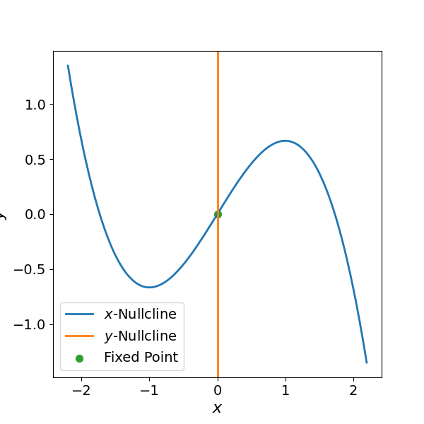
Figure 1:Phase plane portrait of the van der Pol oscillator. Nullclines are shown as thick red lines, with the x-nullcline given by and the y-nullcline along the vertical axis . The lone fixed point is located at the origin (0,0).
To analyze stability, we compute the Jacobian matrix of the system and evaluate it at the fixed point. The Jacobian of the 2-dimensional van der Pol model is given by:
Evaluating at the fixed point yields
The characteristic equation results in the eigenvalues:
The corresponding eigenvectors are:
The stability and qualitative nature of the origin depend entirely on the parameter :
Unstable Spiral (): The eigenvalues are complex conjugates with a positive real part (). Trajectories spiral outward from the origin.
Unstable Node (): The eigenvalues are real and positive. Trajectories move directly away from the origin.
In the high-damping limit (), the eigenvalues exhibit a significant separation in scale: and . This disparity suggests that all trajectories in the neighborhood of the origin are repelled with extreme speed along the direction of the principal eigenvector , which lies almost parallel to the -axis. This mathematical “repulsion” is what initially drives the system toward the lateral branches of the cubic nullcline, setting the stage for relaxation oscillations.
Existence of a limit cycle
The global dynamics of the van der Pol oscillator are defined by the tension between local instability and global boundedness. As shown in the phase portraits (Fig. Figure 2), trajectories originating far from the equilibrium are forcefully “corralled” toward the -nullcline to then follow it in the direction of the steady state. Conversely, as established in our stability analysis, the fixed point at the origin is a repeller, pushing nearby trajectories outward.To prove that these dynamics result in a periodic oscillation, we invoke the Poincaré-Bendixson Theorem. In a two-dimensional system, if a trajectory is confined to a closed, bounded region of the phase plane (a “trapping region”) and that region contains no stable fixed points, the trajectory must asymptotically approach a periodic orbit—a limit cycle. For the van der Pol oscillator, the nonlinear damping term acts as a restorative force that prevents trajectories from escaping to infinity, while the unstable origin prevents them from settling at equilibrium.Unlike the centers found in simple harmonic oscillators, which possess an infinite family of possible orbits depending on initial energy, the van der Pol limit cycle is isolated. This means that regardless of the initial conditions, the system will eventually settle into a unique, self-sustained periodic solution. If a stable limit cycle is perturbed, the system inherently “self-corrects,” returning to the same closed loop. This mathematical robustness explains why the van der Pol model is a cornerstone for describing reliable biological rhythms, such as the rhythmic firing of neurons or the beating of a heart.
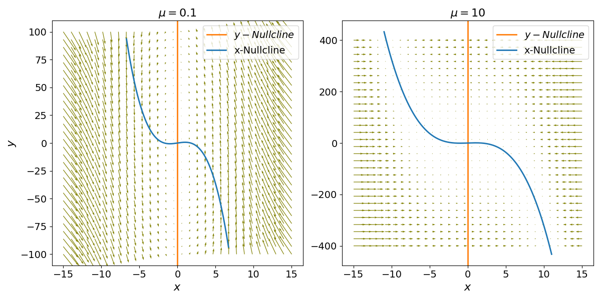
Figure 2:Phase portraits of the van der Pol oscillator for parameter values and , overlaid with nullclines (thick red lines). Arrows indicate vector field flow.
Relaxation Oscillations
In the high-damping limit where , the van der Pol oscillator transforms into a fast-slow system. By examining the Liénard transformation equations, we see that the velocity of the variable is scaled by , while the velocity of is scaled by . This disparity creates two distinct regimes of motion:
The Fast Jump (Horizontal Motion)
Because is proportional to , any deviation from the -nullcline () results in near-instantaneous horizontal movement. As shown in the phase portrait, trajectories starting anywhere in the plane “snap” horizontally toward the stable lateral branches of the cubic nullcline. During these episodes, the slow variable remains virtually constant.
The Slow Drift (Vertical Crawling)
Once the trajectory reaches a lateral branch, the “fast” force vanishes, and the system is governed by the “slow” dynamics of . The trajectory then “creeps” along the nullcline:
Left Branch (): Since is negative, , and the trajectory slowly descends toward the local minimum.
Right Branch (): Since is positive, , and the trajectory slowly ascends toward the local maximum.
The Relaxation Cycle
The oscillation is sustained by a sequence of “jumps” and “drifts”:
Upon reaching the local minimum of the left branch, the system loses its stable support. The fast dynamics take over, causing a horizontal “jump” to the right branch.
Conversely, at the local maximum of the right branch, the system “jumps” back to the left branch.
This alternation between sluggish progression along the branches and explosive jumps between them defines the relaxation oscillation. Unlike the smooth, sinusoidal wave of a harmonic oscillator, the relaxation oscillator produces a “shark-tooth” or pulsed waveform, which more accurately models non-linear phenomena like the firing of a neuron or the snapping of a mechanical governor.
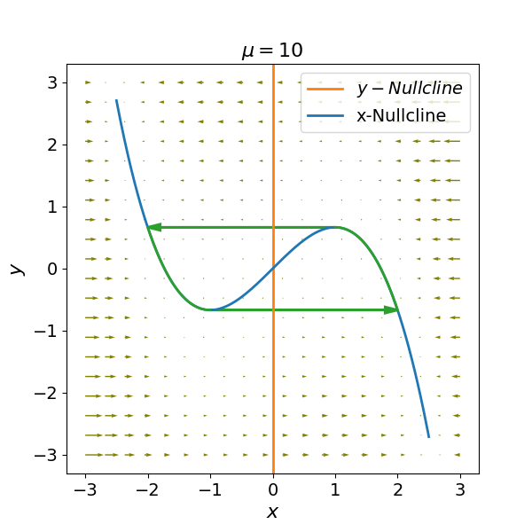
Figure 3:Phase portrait for illustrating relaxation oscillations. Thick blue lines trace a possible oscillation trajectory, rapidly switching between lateral branches (thin red lines) of the -nullcline at local minima/maxima and slowly creeping along branches. Arrows indicate vector field flow.
Discussion
In this chapter, we have introduced and analyzed the dynamics of the van der Pol oscillator. This model, developed by Balthasar van der Pol in 1926, marked the first appearance of the concept of relaxation oscillations in physics and mathematics. By incorporating a nonlinear damping term into the harmonic oscillator equation, van der Pol was able to capture a peculiar oscillatory phenomenon characterized by alternating episodes of rapid change and slow progression between stable solutions.
The relaxation oscillations exhibited by the van der Pol system in the limit of large damping parameter distinguishes it fundamentally from conventional harmonic motion. This characteristic oscillatory behavior arises from the system’s tendency to rapidly approach one lateral branch of the -nullcline before abruptly switching to the other branch at local extremes.
Historically, the van der Pol oscillator played a pivotal role in conceptualizing relaxation oscillations and establishing them as a unique class of self-sustained oscillation distinct from sinusoidal waveforms. Beyond applications in electronics and engineering, van der Pol recognized the potential relevance of relaxation dynamics to biological oscillators underlying rhythmic processes in living organisms.
Indeed, relaxation-type oscillations provide insightful analogies for cyclic behaviors across disciplines. In neuroscience, they have helped quantify electrical spiking patterns in excitable cells like neurons. In cardiovascular physiology, relaxation oscillations resemble pressure-volume loops associated with the heartbeat.
By deriving the first model exhibiting relaxation oscillations, van der Pol laid foundations not only for oscillator theory but also quantitative modeling applications to biological rhythms. The ubiquitous nature of relaxation phenomena continues motivating research at the intersections of physics, engineering, mathematics and the life sciences.
Exercises
Consider the following dynamical system:
Find and characterize the fixed points. Use both analytical and numerical arguments to demonstrate that the system has a limit cycle. Characterize the stability of the limit cycle. Use Liénard’s theorem (https://en.wikipedia.org/wiki/Liénard_equation).
Consider the equation:
where for and for . Using Liénard’s theorem, show that the equivalent two-dimensional system is
with the function defined as
Graph the nullclines. Demonstrate that the system behaves like a relaxation oscillator when and draw the corresponding limit cycle in the phase plane.