11. Local Stability Analysis in 2D Systems - Mathematical Modeling for Life Sciences, A Primer

Abstract

dimensional dynamics emerge from the complex interactions of coupled variables. This chapter generalizes the method of local stability analysis to two-dimensional nonlinear systems modeled by pairs of first-order ordinary differential equations. We introduce the Jacobian matrix as a linear approximation of the system’s behavior near a fixed point and demonstrate how its eigenstructure dictates the evolution of local perturbations. By analyzing the trace ( $\tau$ ) and determinant ( $\Delta$ ) of the Jacobian, we derive a comprehensive classification system that categorizes steady states into nodes, saddles, and spirals. We further connect these analytical criteria to the geometry of the phase plane, providing a visual framework for predicting whether trajectories will converge, diverge, or oscillate. This methodology provides a mathematically rigorous foundation for studying stability in multidimensional systems, an essential skill for modeling complex phenomena across the natural and engineering sciences.

Introduction¶

In a former chapter, we developed the method of local stability analysis to characterize the behavior of steady states in one-dimensional nonlinear dynamical systems. This approach reduces the stability criterion to checking the sign of the slope of the governing function at the steady state. However, many natural and engineered systems are described by models with two or more dimensions that cannot be intuitively visualized or analyzed using one-dimensional techniques. It is therefore necessary to generalize the technique of local stability analysis to higher-dimensional systems described by sets of coupled ordinary differential equations.

In this chapter, we extend the methodology of local stability analysis to two-dimensional nonlinear dynamical systems represented by a pair of coupled ordinary differential equations. While graphical analysis is no longer suitable, the algebraic framework of linearization remains valid. We will see that steady states are now defined as simultaneous solutions to two equations. Linearizing the system dynamics locally yields a $2\times 2$ Jacobian matrix governing small perturbations near the steady state. The matrix’s eigenstructure determines stability and allows a qualitative classification.

By deriving analytical stability criteria from the Jacobian eigenvalues, this approach provides insights into even relatively simple 2D models that are inaccessible through low-dimensional intuition alone. The methodology generalizes directly to higher dimensions through matrix analysis. Local stability analysis thus equips the study of multidimensional dynamical models with a systematic and mathematically rigorous technique.

Steady States in 2D Systems¶

We begin by considering a general two-dimensional dynamical system governed by a pair of first-order ordinary differential equations:

\frac{dx}{dt} = f(x,y), \quad \frac{dy}{dt} = g(x,y),

(1)

where $f(x,y)$ and $g(x,y)$ are smooth functions determining the rate of change of $x$ and $y$ with respect to time $t$ .

In the one-dimensional case studied previously, a steady state or fixed point was defined as a location $x^*$ where the system’s behavior does not change over time. To generalize this concept to two dimensions, we require the system to be stationary at a particular point $(x^*, y^*)$ in the $x$ - $y$ plane. Mathematically, a fixed point $(x^*, y^*)$ satisfies::

\left. \frac{dx}{dt}\right|_{(x^*,y^*)} = 0, \quad \left. \frac{dy}{dt}\right|_{(x^*,y^*)} = 0.

(2)

Substituting into the system of differential equations that defines $dx/dt$ and $dy/dt$ yields:

f(x^*,y^*) = 0, \quad g(x^*,y^*) = 0.

(3)

Therefore, steady states or fixed points in two-dimensional systems are points $(x^*, y^*)$ that are simultaneous solutions to the equations $f(x,y)=0$ and $g(x,y)=0$ .

Local Linearization and Stability Analysis¶

To analyze the stability of a fixed point $(x^*, y^*)$ , we study how small perturbations from this point evolve over time. Let $\delta x = x - x^*$ and $\delta y = y - y^*$ represent deviations of an arbitrary trajectory from the fixed point coordinates. By definition, these perturbations satisfy:

\frac{d \delta x}{dt} = \frac{dx}{dt}, \quad \frac{d \delta y}{dt} = \frac{dy}{dt}.

(4)

Substituting into the ODE system yields: \begin{alight*} \frac{d \delta x}{dt} &= f(x^* + \delta x, y^* + \delta y), \ \frac{d \delta y}{dt} &= g(x^* + \delta x, y^* + \delta y). \end{align*}

Performing a Taylor series approximation truncated to the linear term renders: \begin{alight*} \frac{d\delta x}{dt} &= f_x \delta x + f_y \delta y,\ \frac{d\delta y}{dt} &= g_x \delta x + g_y \delta y \end{align*}

where the partial derivatives are evaluated at the fixed point:

f_x = \left. \frac{\partial f}{\partial x}\right|_{(x^*,y^*)}, \quad f_y = \left. \frac{\partial f}{\partial y}\right|_{(x^*,y^*)}, \quad g_x = \left. \frac{\partial g}{\partial x}\right|_{(x^*,y^*)}, \quad g_y = \left. \frac{\partial g}{\partial y}\right|_{(x^*,y^*)}.

(5)

These linearized equations can be written compactly in matrix form as:

\frac{d \mathbf{\delta r}}{dt} = \mathbf{J} \mathbf{\delta r},

(6)

in which the Jacobian matrix $\mathbf{J}$ contains the partial derivatives, and $\mathbf{\delta r}$ is the perturbation vector.

\mathbf{J} = \begin{bmatrix} f_x & f_y \\ g_x & g_y \end{bmatrix} , \quad \mathbf{\delta r} = \begin{bmatrix} \delta x \\ \delta y \end{bmatrix}.

(7)

Based on the one-dimensional analysis, we expect perturbations to evolve exponentially near the fixed point. Specifically, we make an ansatz that the solution takes the form:

\mathbf{\delta r} = \mathbf{v} e^{\lambda t},

(8)

where vector $\mathbf{v}$ and the scalar parameter $\lambda$ remain to be determined.

Substitution of Eq. (8) into Eq. (6) yields

\lambda \mathbf{v} = \mathbf{J} \mathbf{v}.

(9)

This reveals that for the ansatz to be a valid solution, the parameters $\lambda$ and $\mathbf{v}$ must satisfy the eigenstructure of the Jacobian matrix $\mathbf{J}$ . Specifically, $\lambda$ must be an eigenvalue of $\mathbf{J}$ and $\mathbf{v}$ the corresponding eigenvector.

Since a 2x2 matrix like the Jacobian will generally have two eigenpairs, the complete solution is a superposition of the exponential modes:

\mathbf{\delta r} = C_1 \mathbf{v_1} e^{\lambda t_1} + C_2 \mathbf{v_2} e^{\lambda t_2},

(10)

with $(\lambda_1, \mathbf{v_1})$ and $(\lambda_2, \mathbf{v_2})$ the eigenpairs of $\mathbf{J}$ , while constants $C_1$ and $C_2$ are determined by the initial conditions. We can deduce the asymptotic behavior from Eq. (10): $\mathbf{\delta r}$ decays to zero as $t\to\infty$ if both eigenvalues have negative real parts. In this case, the fixed point is declared locally stable.

Steady-State Classification¶

The eigenstructure relation in Eq. (9) can be expressed as:

(\mathbf{J} - \lambda \mathbf{I}) \mathbf{v} = 0,

(11)

where $\mathbf{I}$ is the 2D identity matrix. This represents a system of two homogeneous linear equations with the components of $\mathbf{v}$ as unknowns. Generally, the only solution to such a system is the trivial solution $\mathbf{v} = \mathbf{0}$ . However, this trivial solution implies $\mathbf{\delta r}(t) = \mathbf{0}$ , meaning that the considered solution is already at the fixed point. This prevents analysis of the stability. A non-trivial solution exists only when the determinant of the coefficient matrix vanishes, i.e. when:

\det(\mathbf{J} - \lambda \mathbf{I}) = 0.

(12)

Expanding this determinant condition gives:

(f_x - \lambda)(g_y - \lambda) - f_y g_x = 0,

(13)

Which can be written compactly in terms of the trace $\tau=f_x+g_y$ and determinant $\Delta=f_x g_y - f_y g_x$ of the Jacobian matrix $\mathbf{J}$ as:

\lambda^2 - \tau \lambda + \Delta = 0.

(14)

Eq. (14) takes the form of a characteristic quadratic polynomial, whose roots correspond to the eigenvalues of the Jacobian matrix $\mathbf{J}$ . The eigenvalues, $\lambda_{1,2}$ , can be explicitly computed by solving the characteristic polynomial:

\lambda_{1,2} = \frac{\tau \pm \sqrt{\tau^2 - 4\Delta}}{2}.

(15)

An analysis of this equation reveals key properties of the eigenvalues based on the values of the trace and determinant. Specifically:

If the determinant $\Delta < 0$ (region I in Fig. Figure 1), then one eigenvalue will be positive while the other is negative, regardless of the sign of the trace $\tau$ .
If $\Delta > 0$ and the discriminant $\tau^2 > 4\Delta$ (regions II and V in Fig. Figure 1), then both eigenvalues will be real and have the same sign as the trace $\tau$ .
If $\Delta > 0$ but the discriminant $\tau^2 < 4\Delta$ , then the eigenvalues form a complex conjugate pair in which $\tau$ is the real part (regions III and IV in Fig. Figure 1). Notably, when the trace $\tau = 0$ , the solutions eigenvalues are purely imaginary numbers.

The above analysis has delineated how the values of coefficients $\Delta$ and $\tau$ determine the possible configurations of the eigenvalues. We now aim to connect these eigenvalue configurations to criteria for classifying the stability of the fixed point.

Regions in the trace-determinant plane delineating qualitative configurations of the Jacobian matrix eigenvalues. The trace \tau and determinant \Delta values determine whether the eigenvalues are real or complex and their relative signs. Region I corresponds to eigenvalues of opposite sign, yielding a saddle node. Regions II and V exhibit real eigenvalues of the same sign, giving rise to unstable and stable nodes, respectively. Regions III and IV contain a complex conjugate eigenvalue pair, resulting in spiral node behavior characterized by rotational motion around the fixed point with exponential decay or growth modulated by the real part of the eigenvalues. 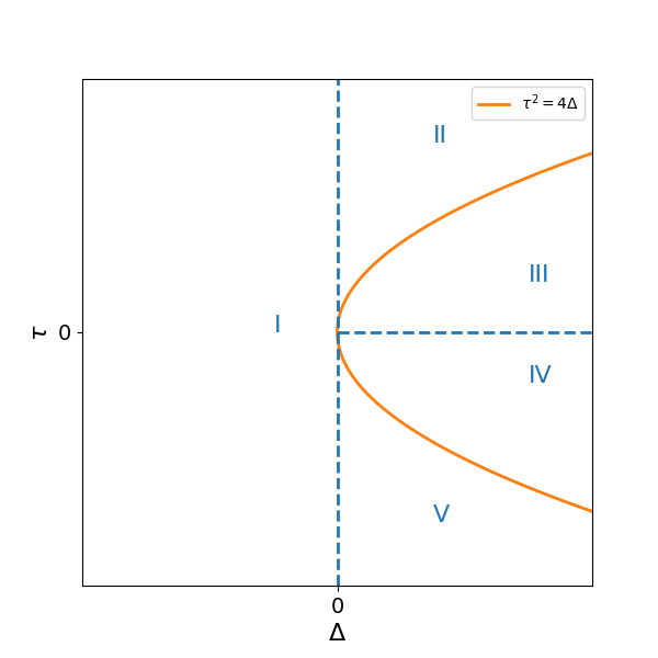— Figure 1:Regions in the trace-determinant plane delineating qualitative configurations of the Jacobian matrix eigenvalues. The trace $\tau$ and determinant $\Delta$ values determine whether the eigenvalues are real or complex and their relative signs. Region I corresponds to eigenvalues of opposite sign, yielding a saddle node. Regions II and V exhibit real eigenvalues of the same sign, giving rise to unstable and stable nodes, respectively. Regions III and IV contain a complex conjugate eigenvalue pair, resulting in spiral node behavior characterized by rotational motion around the fixed point with exponential decay or growth modulated by the real part of the eigenvalues.

Recall that the general solution of the linearized system is given by Eq. (10). When the eigenvectors $\mathbf{v}_1$ and $\mathbf{v}_2$ are unitary and linearly independent, they form a basis of the $\delta x$ - $\delta y$ space, and the terms $C_1e^{\lambda_1t}$ and $C_2e^{\lambda_2t}$ can be interpreted as the coordinates of the perturbation $\mathbf{\delta r}(t)$ at time $t$ in this eigenbasis.

Illustration of phase portraits for representative eigenvalue configurations near a fixed point. Panels: (a) Saddle node (Region I of Fig. ) showing an attracting and a repelling eigendirection; (b) Unstable node (Region II) with trajectories diverging along principal directions; (c) Stable node (Region V) with trajectories converging to the fixed point; (d) Unstable spiral (Region III) displaying outward spiraling motion; (e) Stable spiral (Region IV) displaying inward spiraling motion. 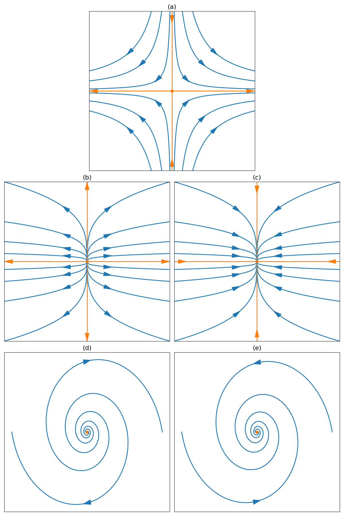— Figure 2:Illustration of phase portraits for representative eigenvalue configurations near a fixed point. Panels: (a) Saddle node (Region I of Fig. Figure 1) showing an attracting and a repelling eigendirection; (b) Unstable node (Region II) with trajectories diverging along principal directions; (c) Stable node (Region V) with trajectories converging to the fixed point; (d) Unstable spiral (Region III) displaying outward spiraling motion; (e) Stable spiral (Region IV) displaying inward spiraling motion.

Considering the full solution as $\mathbf{r}(t) = \mathbf{r^*} + \mathbf{\delta r}(t)$ , we see that $C_1e^{\lambda_1t}$ and $C_2e^{\lambda_2t}$ determine how the linearized solution $\mathbf{r}(t)$ evolves in a reference frame defined by the Jacobian eigenvectors and anchored at the fixed point $\mathbf{r^*}$ .

When the eigenvalues are real, the eigenbasis coordinates $C_1e^{\lambda_1t}$ and $C_2e^{\lambda_2t}$ will exponentially decay or grow over time depending on the sign of the respective eigenvalues. A positive eigenvalue leads to exponential growth of the corresponding coordinate, while a negative eigenvalue implies exponential decay. This characterization of the perturbation growth informs the trajectory sketches shown in Fig. Figure 2 for regions I, II and V of Fig. Figure 1.

The steady state in region I, where one eigenvalue is positive and one is negative, corresponds to a saddle node. Near a saddle node, trajectories will flow away in one eigen-direction and towards the fixed point in the other direction, as illustrated in Figure 2a. A steady state in region II, where both eigenvalues are positive, is referred to as an unstable node. In this case, small perturbations will always grow exponentially, leading trajectories to flow outward from the fixed point in all directions, as shown in Fig. Figure 2b. In region V, where both eigenvalues are negative, the steady state is said to be a stable node. Here, perturbations decay exponentially fast, causing trajectories to converge onto the fixed point from all surrounding points in phase space, as depicted in Fig. Figure 2c.

When the eigenvalues are complex, the linearized system possesses oscillatory behavior near the fixed point. For regions III and IV in Fig. Figure 1, where the trace $\tau$ and determinant $\Delta$ satisfy $\tau^2 < 4\Delta$ , the eigenvalues form a complex conjugate pair $\lambda_{1,2} = \alpha \pm i\beta$ . Substituting this into the general solution of the linearized system in Eq. (10) yields:

\mathbf{\delta r}(t) = C_1\mathbf{v}_1e^{\alpha t}\cos(\beta t) + C_2\mathbf{v}_2e^{\alpha t}\sin(\beta t)

(16)

Observe that the perturbation undergoes rotational motion, with an exponential decay or growth modulated by the real part $\alpha$ of the complex eigenvalues. Since $\alpha = \tau/2$ , where $\tau$ is the trace of the Jacobian matrix, the sign of $\tau$ dictates whether the oscillations decay or grow exponentially over time. Specifically, when $\tau>0$ the real part is positive ( $\alpha>0$ ), corresponding to region III of Fig. Figure 1 where perturbations spiral outward from the fixed point with exponential grow. Conversely, for $\tau<0$ the real part is negative ( $\alpha<0$ ), describing region IV where oscillations spiral inward to the fixed point in a decaying manner. These behaviors are illustrated in Fig. Figure 2d and e.

Discussion¶

In this chapter, we have presented a framework for classifying the behavior near steady state solutions of 2D dynamical systems using linear stability analysis. By analyzing the eigenvalues of the Jacobian matrix ( $\mathbf{J}$ ) evaluated at a fixed point ( $\mathbf{r}^*$ ), we can gain qualitative insight into how perturbations will evolve in the local vicinity of that steady state.

There are three main categories of steady state behavior that emerge based on the signs and types of eigenvalues:

Node: All real eigenvalues lead to exponential decay or growth along principal directions, yielding stable or unstable equilibria.
Saddle: Mixed stability with one growing and one decaying eigenvalue mode. Trajectories flow away along one direction and towards the fixed point along the other.
Spiral: A complex conjugate eigenvalue pair yields stable or unstable rotational motion around the fixed point, with exponential modulation by the real part of the pair.

The stability of nodes and spirals is determined by the sign of the real part of the eigenvalues.

The classifications provided by this local linear stability analysis framework offer powerful insights into the full nonlinear dynamics of the system. Specifically, the local dynamic behavior near steady states allows for a qualitative description of the global behavior of trajectories throughout the phase space. When combined with numerical techniques, this framework enables comprehensive characterization of system dynamics. In the following chapters, we will explore detailed examples that demonstrate these concepts.

Exercises¶

For each one of the following 2-dimensional dynamical systems, find the fixed point, classify their stability, sketch neighboring trajectories, and try to sketch the whole phase portrait:
1. $\dot{x} = y - x, \quad \dot{y} = x^2 -9.$
2. $\dot{x} = 1+y - e^{-x}, \quad \dot{y} = x^2 -y.$
3. $\dot{x} = \sin(y), \quad \dot{y} = \cos(x).$
4. $\dot{x} = y, \quad \dot{y} = x - x^3.$
5. $\dot{x} = yx-16, \quad \dot{y} = x-y^3.$
6. $\dot{x} = 3/(2+y) - x, \quad \dot{y} = 5(x-y).$
7. $\dot{x} = y/(y+1) - x, \quad \dot{y} = 2x - y.$