13. Competitive Lotka-Volterra Model - Mathematical Modeling for Life Sciences, A Primer

Abstract

This chapter presents and analyzes the Lotka-Volterra competitive modeling framework, which describes the population dynamics of two competing species. The framework uses coupled logistic growth differential equations to represent the per capita growth rates of each species, with these rates being reduced by interspecific competition. The chapter examines the steady states of the system and performs phase plane analysis to determine the long-term trajectories defined by different competition coefficient regimes. It also analyzes the stability of the steady states, relating the competitive hierarchies to the resulting community outcomes. Despite the simplifying assumptions inherent in the model, it provides valuable explanatory insights into patterns that conform to Gause’s competitive exclusion principle. By conceptually formulating the interspecific interactions through basic growth and competition functions, the Lotka-Volterra framework demonstrates how even simple conceptual theory can generate ecological understanding of community assembly, focusing on elucidating the underlying mechanisms rather than pursuing precise prediction.

Introduction¶

Intraspecific competition describes interactions between individuals of the same species competing for limited resources. In contrast, interspecific competition characterizes interactions between distinct but ecologically similar species that utilize overlapping resource pools. Past chapters have addressed intraspecific competition mathematically through the logistic model of population growth regulation.

This chapter focuses on interspecific competition, which occurs when multiple species utilize the same limited resources in a single area. As populations of coexisting species continuously interact through competition for necessities like food and shelter, their relative abundances shift in complex ways over time. Describing these population dynamics mathematically provides insights into how competition shapes community structure and long-term species coexistence.

We explore the competitive Lotka-Volterra model, one of the earliest and most influential models developed to study interspecific competition. First introduced independently by Lotka in 1925 and Volterra in 1926, this seminal model formulated competition between species using coupled logistic growth functions. Over a century later, the Lotka-Volterra model remains fundamental to understanding phenomena like competitive exclusion and the conditions permitting diverse communities to coexist simultaneously.

The Competitive Lotka-Volterra Model¶

Lotka and Volterra developed one of the first mathematical formulations of interspecific competition by extending the logistic growth model to multiple interacting species. Their competitive Lotka-Volterra model describes the population dynamics of two species, which we will refer to as species 1 and 2, competing for a shared limiting resource.

The model assumptions are:

Each species exhibits logistic population growth in the absence of the other.
Competition arises through each species reducing the per capita growth rate of the other.

Based on these, the governing equations are:

\begin{align*} \frac{dN_1}{dt} &= r_1N_1\left(1 - \frac{N_1}{K_1} - a_{12}\frac{N_2}{K_2}\right) , \\ \frac{dN_2}{dt} &= r_2N_2\left(1 - \frac{N_2}{K_2} - a_{21}\frac{N_1}{K_1}\right), \end{align*}

(1)

where:

$N_1$ and $N_2$ are the population sizes of species 1 and 2.
$r_1$ and $r_2$ are the intrinsic growth rates.
$K_1$ and $K_2$ are the carrying capacities.
$a_{12}$ and $a_{21}$ are the interspecific competition coefficients.

This pair of coupled nonlinear ordinary differential equations represent the simplest mathematical model capturing the dynamics of competing populations based on limiting resources. We will analyze its properties and implications in subsequent sections.

It is convenient to non-dimensionalize the model by introducing the following scaling:

n_1 = N_1/K_1, \quad n_2 = N_2/K_2, \quad \tau = r_1t.

(2)

This scales population sizes relative to the corresponding carrying capacities and time relative to the intrinsic growth rate of species 1. Substituting these into the original model equations gives:

\begin{align*} \frac{dn_1}{d\tau} = n_1(1 - n_1 - a_{12} n_2), \\ \frac{dn_2}{d\tau} = \rho n_2(1 - n_2 - a_{21} n_1), \end{align*}

(3)

with $\rho = r_2/r_1$ .

Analysis of the Non-Dimensional Model¶

We now analyze the dynamics and behavior of the non-dimensional competitive Lotka-Volterra model derived in the previous section. We first examine the steady of the system, found by setting the derivatives in (3) equal to zero and solving the resulting system of algebraic equations. This gives four possible fixed points:

\begin{align*} E_1 &= (0,0), & E_2 &= (1,0), \\ E_3 &= (0,1), & E_4 &= \left(\frac{1-a_{21}}{1-a_{12}a_{21}}, \frac{1-a_{12}}{1+a_{12}a_{21}}\right). \end{align*}

(4)

The fixed points $E_1$ , $E_2$ , and $E_3$ correspond to boundary equilibria representing the extinction of one or both species. Specifically, $E_1$ is the point of double extinction, $E_2$ is the extinction of species 2, and $E_3$ is the extinction of species 1.

The point $E_4$ is an interior equilibrium where both species can potentially coexist. Notably, $E_4$ exists in the positive quadrant where population sizes are greater than zero only when the interspecific competition coefficients satisfy either $a_{12}, a_{21} < 1$ or $a_{12}, a_{21} > 1$ .

To analyze the stability of the equilibrium points, we compute the Jacobian matrix of the system defined by Eq. (3). Taking the partial derivatives, the Jacobian is:

J = \begin{bmatrix} 1-2n_1-a_{12}n_2 & -a_{12} n_1 \\ -\rho a_{21}n_2 & \rho(1-2n_2-a_{21} n_1) \end{bmatrix} .

(5)

Evaluated at each equilibrium point $E_i$ , the Jacobian matrix $J(E_i)$ characterizes the linearized behavior near that point. The stability type is determined by the eigenvalues of each $J(E_i)$ matrix.

Evaluating the Jacobian at the equilibrium point $E_1=(0,0)$ gives:

J(E_1) = \begin{bmatrix} 1 & 0 \\ 0 & \rho \end{bmatrix} .

(6)

As this is a diagonal matrix, its eigenvectors are aligned with the $n_1$ and $n_2$ axes. The corresponding eigenvalues are 1 and $\rho$ . Since both eigenvalues are positive, the Jacobian evaluation indicates that $E_1$ is an unstable node, where small perturbations will drive the populations away from the double extinction equilibrium.

The Jacobian evaluated at $E_2$ gives

J(E_2) = \begin{bmatrix} -1 & -a_{12} \\ 0 & \rho(1-a_{21}) \end{bmatrix} .

(7)

One of its eigenvectors is aligned with the $n_1$ axis and its corresponding eigenvalue is -1. The other eigenvector is

\left(\frac{a_{12}}{\rho(a_{21}-1)-1}, 1\right),

(8)

while its associated eigenvalue is $\rho(1-a_{21})$ . Therefore, when $a_{21}>1$ , this eigenvalue is negative and the fixed point $E_2$ is a stable node, representing the stable extinction of species 2. Contrarily, when $a_{21}<1$ the eigenvalue is positive and $E_2$ is an unstable node, meaning small perturbations will drive the system away from the extinction of species 2. In summary, the stability of the fixed point where only species 1 survives depends on the competitiveness of species 2, represented by the parameter $a_{21}$ .

The Jacobian evaluated at $E_3$ is:

J(E_3) = \begin{bmatrix} \rho(1-a_{12}) & 0 \\ -a_{21} & -1 \end{bmatrix}.

(9)

The eigenvector aligned with the $n_2$ axis has an eigenvalue of -1. The other eigenvector is

\left(1, \frac{a_{21}}{\rho(a_{12}-1)-1} \right),

(10)

with associated eigenvalue $\rho(1-a_{12})$ . Therefore, when $a_{12}>1$ this eigenvalue is negative and $E_3$ is a stable node, representing the stable extinction of species 1. However, when $a_{12}<1$ the eigenvalue is positive and $E_3$ is an unstable node, meaning small perturbations will drive the system away from the extinction of species 1. Analogous to $E_2$ , the stability of the fixed point where only species 2 survives depends on the competitiveness of species 1, given by the parameter $a_{12}$ .

The Jacobian at the interior coexistence equilibrium $E_4$ is:

J(E_4) = \frac{1}{1-a_{12}a_{21}} \begin{bmatrix} a_{12}-1 & a_{12} (a_{12}-1) \\ \rho a_{21} (a_{21}-1) & \rho(a_{21}-1) \end{bmatrix}.

(11)

The stability of $E_4$ depends on the eigenvalues of $J(E_4)$ , which are given by:

\lambda_{1,2} = \frac{\tau \pm \sqrt{\tau^2 - 4\Delta}}{2},

(12)

where the trace $\tau$ and determinant $\Delta$ are:

\tau = \frac{(a_{12}-1)+\rho(a_{21}-1)}{1-a_{12}a_{21}}, \quad \Delta = \frac{\rho(a_{12}-1)(a_{21}-1)}{1-a_{12}a_{21}}

(13)

It can be shown that:

\tau^2 - 4\Delta = \frac{[(a_{12}-1)+\rho(a_{21}-1)]^2 + 4\rho a_{12}a_{21}(a_{12}-1)(a_{21}-1)}{(1-a_{12}a_{21})^2}

(14)

Since $E_4$ only exists in the positive quadrant when $a_{12},a_{21}<1$ or $a_{12},a_{21}>1$ , this further implies that the eigenvalues are real. If $\Delta>0$ , the eigenvalues have the same sign as $\tau$ , while one is positive and one negative otherwise. Therefore, $E_4$ is a saddle node when $a_{12},a_{21}>1$ because $\Delta<1$ , but a stable node when $a_{12},a_{21}<1$ since $\Delta>0$ and $\tau<0$ .

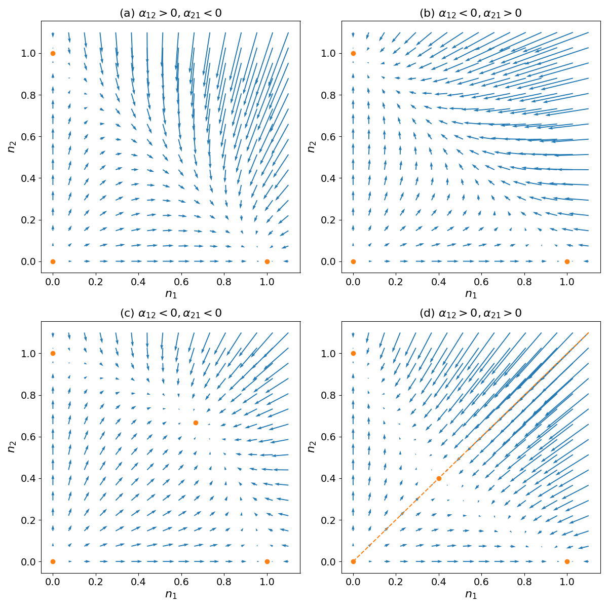
Qualitative behavior of the competitive Lotka-Volterra model in the four regimes defined by the competition coefficients a_{12} and a_{21} — Figure 1:Qualitative behavior of the competitive Lotka-Volterra model in the four regimes defined by the competition coefficients $a_{12}$ and $a_{21}$

The previous analysis reveals four possible long-term scenarios based on the competition coefficients $a_{12}$ and $a_{21}$ , as illustrated in Fig. Figure 1:

When $a_{12} > 1$ and $a_{21} < 1$ , fixed point $E_2$ is the sole stable steady state. In this case, species 1 dominates competition and excludes species 2 in the long run for nearly all starting population levels.
Conversely, when $a_{12} < 1$ and $a_{21} > 1$ , $E_3$ is the only stable steady state. Now species 2 is competitively superior and drives species 1 extinct in the long run.
When $a_{12}$ and $a_{21}$ are both less than 1, $E_4$ represents the sole stable steady state. Here, interspecific competition is weak enough to allow the long-term coexistence of both species for most initial conditions.
Finally, if $a_{12}$ and $a_{21}$ both exceed 1, the extinction equilibria $E_2$ and $E_3$ become stable, creating a bistable system. In this case, the phase plane separates into two basins of attraction defined by a separatrix running through $E_1$ and $E_4$ . Populations beginning in either basin asymptotically approach either the $E_2$ or $E_3$ equilibrium exclusively.

The results of this model analysis have important implications for understanding competitive interactions and community assembly in ecological systems. When interspecific competition is strong, meaning one species is highly dominant over the other, the model predicts that stable coexistence is not possible long-term. The inferior competitor will be excluded from the community. This upholds Gause’s principle of competitive exclusion, which states that no two species can occupy the same niche indefinitely if competing for the same limiting resources.

However, when interspecific competition is weak or mutualistic, the model indicates stable coexistence may occur. Only under conditions of weak resource overlap or facilitation between species can a diverse competitive community persist over generations. This provides insight into how biodiversity is maintained; strong niche differentiation or weak competitive effects allow multiple similar species to stably co-occupy an area together. Overall, the results tie competitive hierarchies directly to potential long-term diversity outcomes, deepening our comprehension of community structure and dynamics.

Discussion¶

While simple and stylized, the competitive Lotka-Volterra model yields important insights into interspecific interactions and their implications for community organization. By capturing the essential dynamics of competing populations through logistic growth and competitive reductions to per capita growth rates, the model provides a mathematical framework for exploring how competition shapes long-term community outcomes.

Despite many unrealistic assumptions, such as constant competition coefficients and symmetrical interspecific effects, the Lotka-Volterra model successfully describes the four qualitative behaviors that can emerge from competitive interactions. These regimes, distinguished by the relative competitive abilities of each species, predict different long-term fates ranging from coexistence to exclusion. In this way, the model functions well as an abstract, conceptual explanatory model rather than a quantitatively predictive one.

Explanatory models like Lotka-Volterra aim to provide mechanistic understanding of natural phenomena, rather than detailed forecasts of real populations. They distill the essence of a process into mathematical terms to investigate general principles and properties. While simplifying assumptions neglect ecological complexities, this allows revealing underlying dynamics that may otherwise remain obscure. The insights generated can then guide more realistic, data-driven modeling as our comprehension progresses.

Naturally, limitations arise from unrealistic assumptions. Despite this, the Lotka-Volterra model fulfills its purpose of building foundational understanding rather than accurate prediction for any specific system. Its enduring usefulness demonstrates the power of conceptual models to advance ecology conceptually. Overall, the Lotka-Volterra model exemplifies how simple theory can provide explanatory insights that stimulate new hypotheses and guide more sophisticated modeling.

Exercises¶

Consider the following example of competition between species. Find the fixed points, determine their stability, plot representative trajectories in the phase plane, and identify the basins of attraction for each stable fixed point:
- $\dot{x}=x(3-2x-y), \quad \dot{y}=y(2-x-y).$
Consider the following example of competition between species. Find the fixed points, determine their stability, plot representative trajectories in the phase plane, and identify the basins of attraction for each stable fixed point:
- $\dot{x}=x(3-2x-y), \quad \dot{y}=y(2-x-y).$
Consider the following model of interaction through competition:
- $\dot{N}_1=r_1 N_1-b_1 N_1 N_{2}, \quad \dot{N}_2=r_2 N_2-b_2 N_1 N_2$ .
Why is this model less realistic than the Lotka-Volterra model? Normalize the model to reduce the number of parameters and analyze it completely: find the fixed points, study their stability, draw the trajectories in the phase plane, and discuss the results.
For the following 2-dimensional dynamical system, plot the bifurcation diagrams showing the equilibrium states ( $x^*$ and $y^*$ ) as functions of the parameter $r$ . Use distinct line styles to differentiate between stable and unstable fixed points:
- $\dot{x} = x(1-x-y/2), \quad \dot{y} = y(1-y-rx)$ .
Identify the type of bifurcation and the critical value $r_c$ at which it occurs. Note: Consider only $x, y, r > 0$ . What are the results implications in the context of the competitive Lotka-Volterra model? l? petitive Lotka-Volterra model?