9. Extending the logistic model - Mathematical Modeling for Life Sciences, A Primer

Abstract

While the standard logistic model accounts for resource limitation, real-world populations are often subjected to external stressors and complex social dynamics that can lead to abrupt collapses. This chapter extends the logistic framework to incorporate two critical biological realities: increased density-independent mortality and the Allee effect. Through these extensions, we move beyond simple convergence to carrying capacity and introduce the fundamental concepts of bifurcation theory and bistability. We demonstrate how rising mortality can trigger a transcritical bifurcation, where a population’s persistence is suddenly exchanged for certain extinction. Furthermore, we show how the Allee effect creates a survival threshold, leading to a system with two stable attractors. By analyzing these models, we gain a mechanistic understanding of “tipping points”—thresholds where minor changes in environmental conditions or population density can result in irreversible shifts in ecological viability.

Increased mortality¶

Up to this point, our logistic population model has assumed that the effective growth rate (the difference between the growth and death rates) is a linearly decreasing function of the population size. In some circumstances, environmental factors unrelated to population density, such as stressors or resource limitation, can elevate mortality. To incorporate this effect, we modify the logistic differential equation. Specifically, we add a term representing density-independent background mortality:

\frac{dN}{dt} = rN(1-N/K) - aN.

(1)

Here, the parameter $a \geq 0$ controls the strength of increased background mortality. When $a=0$ , this model reduces to the basic logistic equation.

To perform a local stability analysis, we first rewrite the logistic differential equation, Eq. (1), in the general form:

\frac{dN}{dt} = f(N),

(2)

where $f(N)=rN(1-N/K)-aN$ . The steady state solutions, also known as fixed points, are given by values of $N$ that satisfy $f(N)=0$ . This yields two fixed points: the extinction state $N^*_1=0$ , and the non-zero equilibrium $N^*_2=K(r-a)/r$ .

To determine stability, we calculate the derivative of the function $f(N)$ to obtain the slope at each fixed point. The derivative is:

f'(N) = (r-a) - \frac{2rN}{K}.

(3)

Evaluating $f'$ at the two fixed points gives: $f'(N_1^*)=r-a$ and $f'(N_2^*)=a-r$ . This reveals that when $a<r$ , the extinction state $N_1^*$ is unstable while the positive equilibrium $N_2^*$ is stable. However, when the mortality rate exceeds the intrinsic growth rate ( $a>r$ ), the stability of the fixed points switches; now the extinction state is stable, whereas the non-zero state $N_2^*$ becomes unstable.

Geometrically, we can gain insight into this transition by visualizing how the fixed points vary with the mortality rate parameter $a$ , as illustrated in Fig. Figure 1. As $a$ increases through the critical value of $r$ , the two fixed points collide at $a=r$ and trade stability. Topologically, this behavior corresponds to a transcritical bifurcation. Physically, it indicates that beyond a threshold level of background mortality, high death rates outweigh new births even at very low population sizes, thereby preventing the population from persisting over long-term. The bifurcation analysis thus provides a framework for understanding how environmental stresses influence population viability through changes in demographic rates.

Bifurcation diagram showing how the two steady state solutions, population extinction (N_1^*) and the positive equilibrium population size (N_2^*), vary dynamically with changes to the background mortality rate parameter (a). The extinction fixed point is depicted with orange lines, while the positive equilibrium is shown in blue. Stable steady states are depicted with solid lines, and unstable states with dashed lines. As a increases beyond the critical threshold value r, equivalent to the intrinsic growth rate, the fixed points intersect at the transcritical bifurcation point. This bifurcation signifies the exchange of stability between the two solutions, where population persistence loses stability and extinction gains stability with further increases in environmental mortality. 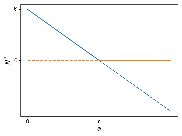— Figure 1:Bifurcation diagram showing how the two steady state solutions, population extinction ( $N_1^*$ ) and the positive equilibrium population size ( $N_2^*$ ), vary dynamically with changes to the background mortality rate parameter ( $a$ ). The extinction fixed point is depicted with orange lines, while the positive equilibrium is shown in blue. Stable steady states are depicted with solid lines, and unstable states with dashed lines. As $a$ increases beyond the critical threshold value $r$ , equivalent to the intrinsic growth rate, the fixed points intersect at the transcritical bifurcation point. This bifurcation signifies the exchange of stability between the two solutions, where population persistence loses stability and extinction gains stability with further increases in environmental mortality.

This model exhibits the first bifurcation encountered in this textbook. It is therefore worthwhile to discuss bifurcations in more detail. By definition, a bifurcation refers to a qualitative change in dynamical behavior that can emerge from small perturbations to parameter values. Specifically, at a bifurcation point the number and/or stability properties of fixed point solutions may abruptly shift. Some common types of bifurcations include:

Saddle-node bifurcation: this occurs when two fixed points coalesce and annihilate one another.
Transcritical bifurcation: a stable and unstable fixed point exchange stability at the critical parameter value.
Pitchfork bifurcation: a single fixed point loses stability, splitting into three solutions of which two are stable.

Bifurcations are significant because they delineate boundaries between distinct qualitative solution behaviors attainable within a model. Identifying these transition points provides insight into how sensitive model predictions are to perturbations of the governing equations.

In the modified logistic population model presented here, the bifurcation that occurs with rising background mortality is of the transcritical type. This bifurcation demarcates how increasing non-density dependent death rates can irreversibly drive the population to extinction once they surpass the capacity for growth. Specifically, as mortality rises past the critical threshold equal to the intrinsic per capita growth rate, the transcritical bifurcation causes the stable fixed point solution representing long-term population persistence to exchange stability with the unstable extinction point. Consequently, above this bifurcation value, mortality dominates reproduction even at very low densities throughout the entire parameter space. This example demonstrates that environmental stressors can precipitate a population tipping point between ongoing viability versus extinction by tilting the demographic balance through small alterations to basic rates of birth and death. Identifying such bifurcation-defined thresholds provides insight into how susceptible population persistence is to fluctuations in underlying biological parameters.

Allee Effect¶

Small populations face additional hurdles that threaten their long-term sustainability. This phenomenon, known as the Allee effect, arises due to difficulties finding mates and engaging in beneficial forms of cooperation at very low densities, resulting in decreased per capita growth. To represent this intrinsic difficulty in the logistic model, we introduce an Allee term as follows:

\frac{dN}{dt} = rN\left(1-\frac{N}{K}\right)\left(\frac{N}{A}-1\right).

(4)

In this formulation, parameter $0 < A < K/2$ represents a population threshold below which the effective per capita growth rate becomes negative, meaning that deaths exceed births.

Let us analyze Eq. (4) in its general functional form, $\dot{N}=f(N)$ , where $f(N)=rN(1-N/K)(N/A-1)$ . The form of this function $f(N)$ is depicted graphically in Fig. Figure 2. As seen in the figure, $f(N)$ intersects the horizontal axis at three distinct points, indicating the presence of three steady state solutions: population extinction at $N_1^*=0$ , an interior equilibrium at $N_2^*=A$ , and a second fixed point at the carrying capacity $N_3^*=K$ . Furthermore, the derivatives satisfy $f'(N_1^*)<0$ , $f'(N_2^*)>0$ , and $f'(N_3^*)<0$ . This confirms that $N_1^*$ and $N_3^*$ are stable nodes, while $N_2^*$ is an unstable saddle point.

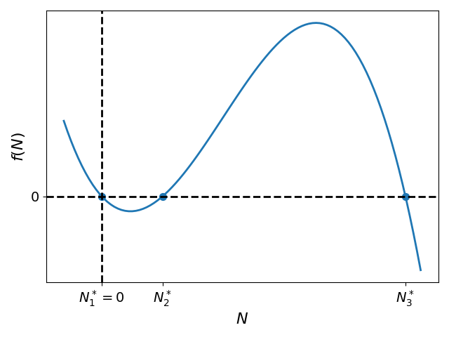
Graphical depiction of the function f(N)=rN(1-N/K)(N/A-1) describing per capita growth rate in the Allee effect model-Eq. {eq}`eq:09.02 — Figure 2:Graphical depiction of the function $f(N)=rN(1-N/K)(N/A-1)$ describing per capita growth rate in the Allee effect model-Eq. {eq}`eq:09.02

The existence of two locally stable fixed points separated by an unstable steady state in this modified logistic model, namely the extinction state $N_1^*$ and the positive carrying capacity $N_3^*$ , gives rise to bistability in the system’s dynamics. Biologically, bistability implies that the population can persist indefinitely at either stable state of extinction or carrying capacity, with the final outcome dependent on initial conditions. Stochastic fluctuations may cause the population to randomly switch between attractors.

The logistic equation exhibiting an Allee effect is the first example in this textbook to demonstrate bistability. As a key feature of nonlinear systems, bistability will emerge again in other examples throughout this textbook, continually deepening our understanding of its consequences for real-world ecological and biological systems.

Discussion¶

In this chapter, we explored two extensions to the basic logistic population growth model: increased background mortality and an Allee effect. By incorporating density-independent mortality through an additional death term, the model exhibited a transcritical bifurcation whereby changes to the mortality rate could precipitate a population tipping point between ongoing viability and extinction. This demonstrated how environmental stresses may trigger abrupt, irreversible transitions in population state through subtle parameter changes.

Incorporating an Allee effect produced bistability, in which the population could persist indefinitely at either the extinction or carrying capacity stable states depending on initial conditions. Bistability highlights the sensitivity of ecological systems to random perturbations, with the potential for sudden shifts between alternative community states. It is a nonlinear phenomenon with significant implications for population persistence and community resilience.

More broadly, this chapter demonstrated the utility of dynamical systems theory and tools like bifurcation analysis for gaining mechanistic understanding of population viability. Such approaches aim to tease apart how multiplicative interactions between intrinsic biological processes and density-dependent feedbacks shape complex, often counterintuitive population dynamics over time.

Exercises¶

Chapter 9¶

In the logistic model, the effective growth rate $\dot{N}/N$ is maximal at $N=0$ . An alternative way to introduce the Allee effect is to have $\dot{N}/N$ reach its maximum at some intermediate value between 0 and the carrying capacity.
Show that $\dot{N}/N = r - a(N-b)^2$ satisfies the above definition under specific conditions for $a$ , $b$ , and $r$ . What are these conditions?
Identify the system’s fixed points and classify their stability.
Compare the solutions of this model with those of the logistic model.
For the following dynamical systems, plot the bifurcation diagram showing the equilibrium states ( $x^*$ ) as a function of the parameter $r$ . Use distinct line styles to differentiate between stable and unstable fixed points. For each system, identify the type of bifurcation and the critical value $r_c$ at which it occurs. Note: Consider only $r > 0$ .
$\dot{x} = 1+r x+x^2,$
$\dot{x} = x - rx (1-x),$
$\dot{x} = r x+4 x^3,$
$\dot{x} = r x-4 x^3,$
$\dot{x} = (x + 1)(x - 1) + r,$
$\dot{x} = x((x+1)^2 - r).$